Getting Started

1. Getting Started#

This chapter introduces fundamental concepts for working with code. We begin with the Unix command line and environment management, after which we will turn to an overview of the Python programming language.

Prerequisites: If you are using Windows, install Git for Windows. It comes with Git Bash, a Unix-style command-line interface
Credits: Portions of this chapter are adapted from the UC Davis DataLab’s Introduction to the Command Line, Introduction to Remote Computing, and Python Basics

1.1. Command Line Basics#

Most modern coding platforms follow the conventions of mainstream computing, using a graphical user interface (GUI) to display information and accept user input. But there is still real value in knowing the basics of the command-line interface (CLI), which relies solely on text input. Learning how to use the CLI will teach you a great deal about how your computer works, and there are still several instances where CLIs are the only point of access to a system.

The CLI contains three main parts:

A terminal: an environment you use to send/receive information to/from your computer
A shell: a program that executes commands you enter into the terminal
The command line: where you enter the commands that the shell executes

As we move through this chapter, keep one key thing in mind: a CLI is just another mode of interaction with your computer. Everything you can access through a windowing system on a GUI is also accessible with a CLI.

1.1.1. Launching a command-line interface#

MacOS comes with a pre-installed CLI called Terminal. To launch it, go to:

Applications -> Utilities -> Terminal

Windows users will use Git Bash. To launch it, do the following:

Windows Start Menu -> search "Git Bash"

Or:

Windows Start Menu -> Programs -> Git Bash

You should see something like this when your CLI launches:

A command-line interface window

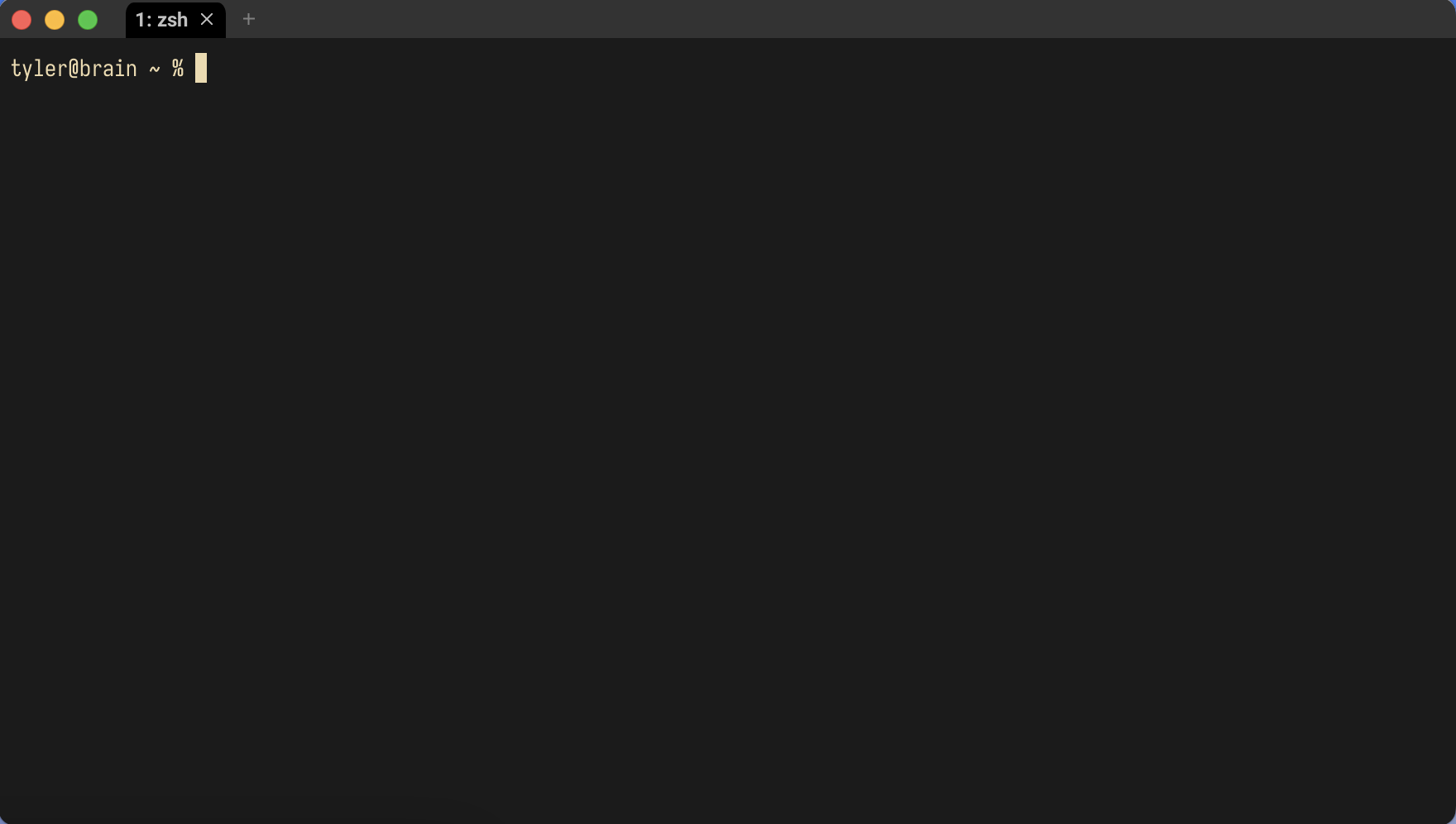
The window above shows a basic command line with a prompt. A prompt is an input field where you type your commands, and it is prepended with useful information about your computer:

First, tyler@brain tells us the current user (tyler) and the current computer (brain). That may seem like redundant information, but with the command line it’s possible to log in to other computers
The prompt also tells us where we are on this computer’s file system. Right now we are at ~. We’ll discuss what this symbol means later. For now, just keep in mind that this is where you should look to get your bearings
Finally, we see %. It is an indicator that the CLI is waiting for input

Tip

In the following sections, we will display CLI commands by prepending them with an indicator character, $. You do not need to type this character yourself, it’s just to signal that a cell shows a command.

1.1.2. Input and interactions#

Time to enter some commands. This is simply a matter of typing them in after the prompt and pressing Return/Enter.

For example, echo will print back to screen any text that you supply the command:

$ echo "Hello world!"

Hello world!

You can see what files and folders are in your current location with ls (“list”):

$ ls

_build      _config.yml _toc.yml    chapters    data        env         img         scratch     src

Send ls the name of a subfolder to show its contents:

$ ls chapters

01_getting-started.md      04_ngram-models.md         07_intro-to-llms.md        index.md
02_python-basics.md        05_vectorization.md        08_bert.md
03_data-analysis-basics.md 06_vector-spaces.md        09_gpt.md

Want more information? Modify the base functionality of ls—or any command—with flags. We do this by adding a dash - and then a letter, or a combination of letters, directly after the dash. Below, we send ls flags to have it show all contents (a) with long-formatted output (l) in a human-readable fashion (h):

$ ls -alh

drwxr-xr-x  13 <username>  staff   416B May 25 01:46 .
drwxr-xr-x   5 <username>  staff   160B May  8 12:58 ..
drwxr-xr-x  14 <username>  staff   448B May 25 01:35 .git
-rw-r--r--   1 <username>  staff    20B Apr 22 15:44 .gitignore
drwxr-xr-x   6 <username>  staff   192B Apr 25 22:01 _build
-rw-r--r--   1 <username>  staff   501B Apr 21 23:23 _config.yml
-rw-r--r--   1 <username>  staff   583B Apr 22 10:10 _toc.yml
drwxr-xr-x  12 <username>  staff   384B May 30 13:00 chapters
drwxr-xr-x  11 <username>  staff   352B May 17 17:16 data
drwxr-xr-x   5 <username>  staff   160B May 30 12:37 img
drwxr-xr-x   5 <username>  staff   160B May 25 01:35 src

Long-formatted output shows you metadata about files and folders, including information about the their owner/group (<username> and staff), their permissions (those strings of r’s, w’s, and x’s), their size, and the last date they were modified. We won’t discuss permissions in depth, but know that they dictate who can read r, write w, and execute x files.

Any file or folder prepended with . in its name will be hidden by default on your computer. But using the all -a flag, as we did above, will show them: ., .., .git, and .gitignore. The first two are special notations for navigating your computer, which we discuss in the next section. The third, .git, is a subfolder that stores version control information about this reader, and .gitignore is a dotfile. Dotfiles often contain various configuration settings that people use to customize their computers. In this case, .gitignore controls what parts of this folder version control should ignore.

1.1.3. Command-line syntax#

Depending on your computer and CLI, the above output may differ slightly, but in general the basic presentation and functionality will be the same. Commands use a space to delimit their different components, and flags are called with - to modify those commands. When put together, we can generalize these components to a command-line syntax:

$ <command> <optional flags> <file/data on which to run the command>

One caveat: since spaces are a meaningful part of the command-line syntax, file names with spaces in them can cause problems. You’ll need to escape these names with \.

This will throw an error:

$ <command> file name.txt

But this will not:

$ <command> file\ name.txt

Be sure to read error messages when you see them. While the CLI is often quite mute, it will do its best to show you what you did wrong when an error arises. Below, for example, the shell explains that it cannot find a command, which actually stems from a typing error:

$ lschapters

zsh: command not found: lschapters

Likewise, here, ls cannot find the requested folder because it does not exist:

$ ls storage

ls: storage: No such file or directory

One last thing about general CLI usage. Sometimes, you need to stop a process immediately. Use CTRL+C to interrupt it. But keep in mind that, for the most part, it isn’t possible to undo a command. Take care to know exactly what you’re running and what you’re running it on, especially as you get acclimated to the CLI.

1.1.4. Getting help#

There are dozens of commands available to you on your computer, and you can install even more. If you’d like to see an overview of some of the most common commands, take a look at Valerie Summet’s Unix cheat sheet.

You can also use man (“manual”). This opens the manual page for another command. Here you will find usage information, including what flags a command accepts.

$ man ls

LS(1)                                            General Commands Manual                                            LS(1)

NAME
     ls – list directory contents

SYNOPSIS
     ls [-@ABCFGHILOPRSTUWabcdefghiklmnopqrstuvwxy1%,] [--color=when] [-D format] [file ...]

DESCRIPTION
     For each operand that names a file of a type other than directory, ls displays its name as well as any requested,
     associated information.  For each operand that names a file of type directory, ls displays the names of files
     contained within that directory, as well as any requested, associated information.

     If no operands are given, the contents of the current directory are displayed.  If more than one operand is given,
     non-directory operands are displayed first; directory and non-directory operands are sorted separately and in
     lexicographical order.

     The following options are available:

<...>

A shortened version of this output is often available by flagging a command with --help. Sometimes, too, you will need to know the version of the command you’re using. You can find this information with --version, or --v.

1.2. Directory Structures#

Remember that a CLI is just another mode of interaction with your computer. This section will solidify that idea by showing you how to navigate your computer’s directory structure, the arrangement and organization of its data.

1.2.1. Paths#

A directory structure is like a map of all the locations you can navigate on your computer. These locations are directories (or folders), and within them are files (chunks of data). Each file has an address on this map, and there is a path that leads to it. The windowing systems of modern computers manage these paths automatically when you click around on your computer, but it’s also possible to navigate on the command line. You’ll just need to specify paths yourself.

In a Unix environment, we do this with the following syntax:

/this/is/a/path/to/your/file.txt

This is called a file path. It threads through multiple directories to point at your desired file, file.txt.

Note

Non-Unix environments, like Windows DOS, use \ instead of /:

C:\this\is\a\path\to\your\file.txt

This is why Windows users had to download Git Bash. It emulates Unix-style functionality on those machines. Generally speaking, the Unix command line is far more pervasive than DOS, so you’ll find yourself using Unix-style commands/syntax more frequently.

1.2.2. Path hierarchies#

A directory structure is hierarchical. Directories are “above” or “below” one another, and it’s crucial to get a sense of this so that you can navigate your computer. In the file path above, every / demarcates a new one of these directory levels.

Use pwd (“print working directory”) to display your current location using the same format:

$ pwd

/Users/tyler/2024_dtl_lm-interpretability

Note that this path begins with /. This is the top-most directory in your computer, called the root. It’s like the trunk of a tree: every directory branches off from it. But, to add some complications, directories can also branch off one another. Whenever you make a new directory, you’ve created another branch in this tree, and this branch is at the same time a branch of root and a branch of whatever directory you’re currently in.

For example, here is the structure of this reader’s data directory:

data
├── datasets
├── models
│   └── bert_blurb_classifier
│       └── final
└── texts
    ├── dickinson
    │   └── poems
    └── nyt
        └── obituaries

See the branching paths?

Note

DOS again diverges from Unix in its representation of the root. For the former, the root is usually called C: or D:, which designates the actual device on which your data is stored.

1.2.3. Absolute vs. relative paths#

No matter the operating system, there are two different ways to specify a file path on the command line. Recall our pwd output above:

$ pwd

/Users/tyler/2024_dtl_llm-interpretability

It starts with root /. When you see a path like this, it’s showing you the full, or absolute, location of a directory or file. By typing out this path, you can navigate directly to this location, regardless of where you are on your computer.

By contrast, a relative path is context-specific. It depends on where you are in your computer’s directory structure. Unix uses shorthand to denote this location:

. denotes the current location in your computer
.. denotes the directory above that location

Remember seeing these earlier with ls -alh? Your computer tracks locations by placing these two symbols in every directory you create. Thus, this enables you to use this shorthand notation to avoid typing out the entire path to a file. This is useful if you’re a ways off from root, or if, for a coding project, you are using files that rely on a specific directory structure, which could be ported to someone else’s computer.

Besides . and .., there is also ~, which we saw in the CLI prompt earlier. This denotes your home directory, which your computer uses to store data and configurations that are specific to you. Use cd (“change directory”) in combination with ~ to return to home, no matter where you are in your computer’s directory structure.

$ cd ~

Take a look at your prompt: it should list out ~ in the location position.

1.2.4. Navigating with a CLI#

Here’s an example of absolute and relative paths. Say you are here:

/here/is/where/you/are/located/in/your/computer
                                       ^^^^^^^^

…and you want to get to located:

/here/is/where/you/are/located/in/your/computer
                       ^^^^^^^

You could use an absolute path:

$ cd /here/is/where/you/are/located

The logic of this path runs like this:

root
└── here
│   └── is
│       └── where
│           └── you
│               └── are
└──────────────────>└── located
                        └── in
                            └── your
                                └── computer

Alternatively, you could use a relative path:

$ cd ../../../

In contrast with the absolute path, the logic of this relative one runs like this:

root
└── here
    └── is
        └── where
            └── you
                └── are
                    └── located
                    ^   └── in
                    │       └── your
                    │           └── computer
                    └───────────────┘

Your relative path would take you three directories up from computer to located. That’s considerably shorter than writing the path out in full, but there’s also a downside: using multiple .. symbols makes it hard to know what the context of the path is, and it’s easy to get confused. So, there’s a trade-off between absolute and relative paths, which you’ll often find yourself making.

Finally, we can move data and directories around on our computers using paths. To move a file, use mv (“move”), which works like so:

$ mv <location/of/file> <location/where/you/want/to/move/the/file>

If we’re in a directory that looks like this:

$ ls

file.txt  subdirectory

…and we’d like to move file.txt into subdirectory, we use:

$ mv file.txt subdirectory

Or, maybe we want to make a new directory inside subdirectory. Use mkdir (“make directory”) to make a new directory, new, which will sit under subdirectory.

$ mkdir subdirectory/new

Now, from our current location, we move file.txt into new.

$ mv subdirectory/file.txt subdirectory/new/file.txt

This is what the directory structure looks like now:

current_location
└── subdirectory
    └── new
        └── file.txt

1.3. Environment Setup#

Processes—applications, background tasks, code, etc.—run on your computer in a computer environment. These environments are collections of hardware, software, and various configurations, and the latter two are portable between computers (ideally). This portability is great for when you get a new computer and want to recreate your current environment, whether by replicating certain settings or installing external software; but the real power of porting environments stems from the ability to freeze them and share them with others.

You’ll often have to do this when writing code, because some people may not have certain pieces of software that you have on your computer. And, as we’ll discuss a little later on, writing code often relies on specific versions of programming language packages, which can conflict with one another—and cause massive headaches. Using an environment manager to encapsulate your setup will help you circumvent such problems and let others run your code as you intended.

1.3.1. Micromamba#

We will use micromamba to manage environments for the work that lies ahead. It allows us to create new virtual environments and install software into them, including different versions of Python and associated packages. micromamba is based on mamba, which is in turn based on conda; the three are drop-in replacements for each another, so when you see discussions about one, know that the topic will likely port over to the others.

The micromamba documentation (linked above) will always feature the most recent version of installation instructions. As of this writing (summer 2024), installing via the script option in a CLI works like so:

$ "${SHELL}" <(curl -L micro.mamba.pm/install.sh)

Running this command will download and install a script. During installation, you’ll be asked a series of questions:

Micromamba binary folder? [~/.local/bin]: Where do you want to install the program? Select the default by pressing Enter/Return
Init shell (bash)? [Y/n]: Configure your shell for micromamba? Enter Y
Configure conda-forge? [Y/n]: Default to the conda-forge repository when searching for packages to install? Enter Y
Prefix location? [~/micromamba]: Where would you like to install environments? The default is under your home directory, which is fine. Press Enter/Return

With these options set, reload your shell to initialize micromamba:

zsh

$ source ~/.zshrc

bash

$ source ~/.bashrc

Tip

You don’t need to run source to initialize micromamba every time you open your CLI. Your CLI actually runs this command when on start up—we just have the program running already.

Now check the version of micromamba:

$ micromamba --version

1.5.8

If you see output like the above, you’re set!

Time to create a new environment. Generally, it’s a good idea to make a new environment for every project. Below, we make one called practice.

$ micromamba create --name practice

Empty environment created at prefix: <path/to/practice>

Use the env list subcommand to list out all environments:

$ micromamba env list

  Name      Active  Path
──────────────────────────────────────────────────────────
  practice          <path/to/micromamba/envs/practice>

Activate an environment with the activate <enviroment> subcommand.

$ micromamba activate practice

Note your prompt. It will update to reflect that you’re in a micromamba environment:

(practice) you@your_computer ~$

Let’s install some software. Below, we install ripgrep, which enables you to search text files in a directory:

$ micromamba install ripgrep

When prompted, enter Y to confirm that you’d like to install the program.

Now, use ripgrep to search for “NLP” in chapters:

$ rg -i "NLP" chapters

chapters/06_vector-spaces.md
 [Natural Language Processing for Data Science][nlp]
[nlp]: https://ucdavisdatalab.github.io/workshop_nlp_reader
reigning metaphor of NLP, a space of this sort is a stand-in for meaning: the
 in the same direction as the first. Most vector operations in NLP use the
to be made available by the Stanford NLP group. It has been trained on a 2014
[glove]: https://nlp.stanford.edu/projects/glove/

chapters/01_getting-started.md
Now, use `ripgrep` to search for "NLP" in `chapters`:
$ rg -i "NLP" chapters
309:all repeated tokens. The result will be a set of in NLP are called **types**:
666:Now, use `ripgrep` to search for "NLP" in `chapters`:
669:$ rg -i "NLP" chapters
673:648:  in the same direction as the first. Most vector operations in NLP use the
676:309:all repeated tokens. The result will be a set of in NLP are called **types**:
679:664:Now, use `ripgrep` to search for "NLP" in `chapters`:
680:667:$ rg -i "NLP" chapters
694:$ rg -i "NLP" chapters
863:machine learning/AI and natural language processing (NLP): most people are
1272:nlp = "natural language processing"
1273:nlp.title()
1279:nlp.count("g")
1294:dir(nlp)
1422:computing, NLP, and machine learning/AI. A full list of them is provided in the
648:  in the same direction as the first. Most vector operations in NLP use the
$ rg -i "NLP" chapters
machine learning/AI and natural language processing (NLP): most people are
nlp = "natural language processing"
nlp.title()
nlp.count("g")
dir(nlp)
computing, NLP, and machine learning/AI. A full list of them is provided in the

chapters/02_python-basics.md
all repeated tokens. The result will be a set of in NLP are called **types**:

chapters/03_data-analysis-basics.md
 [Python Basics][python] and [Natural Language Processing for Data Science][nlp]
[nlp]: https://ucdavisdatalab.github.io/workshop_nlp_reader

chapters/05_vectorization.md
 [Natural Language Processing for Data Science][nlp]
[nlp]: https://ucdavisdatalab.github.io/workshop_nlp_reader

chapters/07_intro-to-llms.md
 [Natural Language Processing for Data Science][nlp]
[nlp]: https://ucdavisdatalab.github.io/workshop_nlp_reader

See how it picked up the very text you’re reading now?

Use the deactivate subcommand to deactivate an environment.

$ micromamba deactivate

Now, if you try to use ripgrep, you’ll get an error:

$ rg -i "NLP" chapters

zsh: command not found: rg

Why the error? You’ve installed ripgrep into a separate environment managed by micromamba, which is sealed off from the rest of your computer.

To see all packages installed in an environment, use list:

$ micromamba activate practice
$ micromamba list

List of packages in environment: "<path/to/micromamba/envs/practice>"

  Name           Version  Build        Channel
────────────────────────────────────────────────────
  _libgcc_mutex  0.1      conda_forge  conda-forge
  _openmp_mutex  4.5      2_gnu        conda-forge
  libgcc-ng      13.2.0   h77fa898_7   conda-forge
  libgomp        13.2.0   h77fa898_7   conda-forge
  ripgrep        14.1.0   he8a937b_0   conda-forge

Why does this list have more than ripgrep? Those are the program’s dependencies, external pieces of software written and released by other programmers that ripgrep uses to run. If you want to use ripgrep, you need those as well, and it’s micromamba’s job to figure out how to manage those dependencies.

For example, micromamba will include them when you export your environment with the env export subcommand:

$ micromamba env export

name: practice
channels:
- conda-forge
dependencies:
- _libgcc_mutex=0.1=conda_forge
- _openmp_mutex=4.5=2_gnu
- libgcc-ng=13.2.0=h77fa898_7
- libgomp=13.2.0=h77fa898_7
- ripgrep=14.1.0=he8a937b_0

Those letter and number combinations after each entry are specific versions, which another person could use to recreate your current environment. That said, sometimes operating system differences complicate versioning, so set the --from-history flag to get only the names of the packages you’ve installed:

$ micromamba env export --from-history

name: practice
channels:
- conda-forge
dependencies:
- ripgrep

Note

If you installed a package with a specific version, e.g.:

$ micromamba install ripgrep=12.1

…the --from-history flag will preserve this:

$ micromamba env export --from-history

name: practice
channels:
- conda-forge
dependencies:
- ripgrep=12.1

Redirect the output of your environment export to a YAML file using >:

$ micromamba env export --from-history > practice.yml

And that way someone can install it on their own computer, using:

$ micromamba env create --file practice.yml

Finally, to remove an environment, deactivate it and run the following:

$ micromamba env remove --name practice

1.3.2. Jupyter Lab#

With an environment manager installed, we turn now to a development environment for writing and running code. There are several applications to choose from; we will use a simple, open-source environment called JupyterLab. JupyterLab runs in your web browser, it’s highly portable and flexible, and it has an integrated notebook interface for writing, documenting, recreating, and running code.

Before we download JupyterLab, we’ll create a new micromamba environment, main. While it’s a good idea to have project-specific virtual environments, using a separate one to run JupyterLab and other such general programs will keep you from re-installing the same software over and over.

$ micromamba env create --name main

Now, we install JupyterLab with micromamba.

$ micromamba activate main
$ micromamba install jupyterlab

To run the application, enter the following in your CLI:

$ jupyter lab

This will open a new tab in your web browser, where JupyterLab will be running:

JupyterLab interface

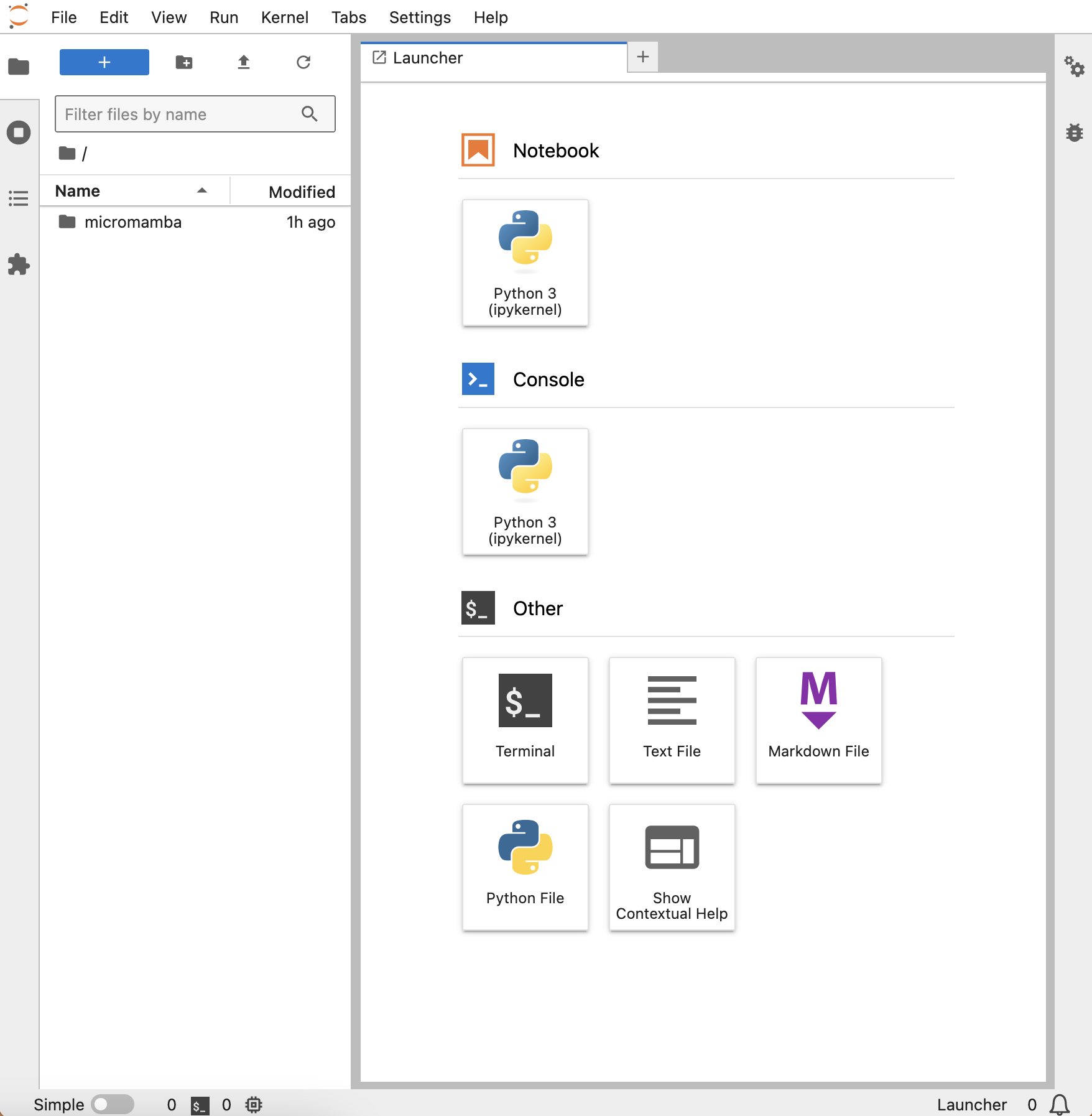
At the left you’ll see a file browser. In the Launcher, there are options to launch coding interfaces (under both Notebook and Console), a terminal, or various text files. To run code, JupyterLab uses kernels. Kernels are associated with specific programming languages, and they allow users to write code in an interactive way. We’ll use a Python kernel, but you can also install ones for R, Julia, and other languages.

It’s also possible to create a kernel for a virtual environment. We’ll do this shortly. But for now, click on the default kernel, Python 3, under Notebook. This will launch a Jupyter notebook. These files support code execution in cells, text formatting via Markdown, image rendering, and more. While programmers typically write their code in plain text files, the interactivity and formatting features of Jupyter notebooks make them highly useful for developing and demonstrating code. That said, unlike plain text files, these files must be rendered in a web browser by Jupyter. There’s no easy way to see their contents otherwise.

1.4. Writing Code in Python#

We will be writing all of our code in Python. It’s a massively popular, general-purpose programming language with big communities of support. For our purposes, most notable among these communities are the ones that support machine learning/AI and natural language processing (NLP): most people are using Python to write this kind of code.

To write Python code in a notebook, click on a cell and type an expression. Expressions are combinations of values, variables, operators, and functions, which Python (and other programming languages) interprets and then evaluates.

Here is a simple expression:

2 + 2

Press Shift + Enter to run it:

2 + 2

Now, try subtraction:

7 - 1

You can write any arithmetic equation in Python using these and other operators. These are symbols that represent common operations for arithmetic, comparison, and logical evaluation. The table below records Python’s arithmetic operators.

Operator	Meaning
`+`	Addition
`-`	Subtraction
`*`	Multiplication
`/`	Division
`%`	Remainder division (modulo)
`**`	Exponentiation

Use parentheses ( ) to create more complicated expressions. Python will evaluate these expressions in the standard order of operations: parentheses, exponentiation, multiplication, division, addition, and then subtraction.

(2 + 2) * (7 - 1)

Technically, there’s no need to add spaces between these expressions, but doing so helps with readability.

(2+2)*(7-1)

1.4.1. Variables#

Below, we calculate the area of a triangle with base 2.5 and height 4:

2.5 * 4 * 0.5

5.0

If we wanted to store the result of this expression for later use, we’d need to assign it to a variable. Create one by writing out the name of the variable and using the assignment operator = to link the variable with an expression.

area = 2.5 * 4 * 0.5

Variables can be any combination of letters, numbers, or underscores _. They cannot start with a number, however, and other symbols are not allowed in their names. When you write code, you’ll find yourself using variables all the time. Not only do they store values; they also make your code more reusable and more readable, and they help you generalize your code beyond specific values.

For example, we can create variables for base and height that allow us to change area with ease:

base = 2.5
height = 4
area = base * height / 2
area

5.0

Want another value? Reassign the variable:

height = 5
area = base * height / 2
area

6.25

Good variable names are descriptive. While these are two perfectly valid variables:

i8 = 4
_a = 5

It would be hard to track what they stand for when you go to use them:

result = (i8 ** 2 + _a ** 2) ** 0.5
result

6.4031242374328485

Let’s clarify:

leg_1 = 4
leg_2 = 5
hypotenuse = (leg_1 ** 2 + leg_2 ** 2) ** 0.5
hypotenuse

6.4031242374328485

In both cases, we calculated the hypotenuse of a right-angled triangle following the Pythagorean theorem, but the second expression makes this much more clear.

1.4.2. Strings#

Python uses different data types to store certain kinds of values. We’ve already used numeric types, but it’s also possible to create strings and logical values.

To create a string in Python, use either single ' or double " quotes:

"I am a string"

'I am a string'

Note that the quotes must match, or you’ll cause an error:

"I am a string'

  Cell In[13], line 1
    "I am a string'
    ^
SyntaxError: unterminated string literal (detected at line 1)

If you want to use quotations inside your string, you need to use a different kind of quotation mark to enclose that string:

"I'm a string"

"I'm a string"

Or, you can escape the string with \. This tells Python to treat the following symbol as if it were just a string, not a special character for the language itself.

'I\'m a string'

"I'm a string"

Note that there is a difference between numeric values and strings that represent values. That is, 1 does not equal "1".

1.4.3. Numbers#

There are two kinds of numeric types In Python, integers and floats. Integers are just whole numbers:

Whereas floats represent decimals:

8.8

8.8

When you perform arithmetic expressions in Python, the language will automatically determine whether the result should be represented as an integer or a float. Here’s an integer result:

5 + 5

And a float:

1 / 3

0.3333333333333333

Both numeric types may be either positive or negative. Use - to create a negative number:

-4

-4

Certain expressions will also produce negative numbers:

8 - 12

-4

1.4.4. Comparisons#

You’ll often need to compare values when you code. Use comparison operators to do so:

Operator	Meaning
`<`	Less than
`>`	Greater than
`<=`	Less than or equal to
`>=`	Greater than or equal to
`==`	Equal to
`!=`	Not equal to

Note that “equal to” uses two equal symbols to distinguish it from the assignment operator =.

Comparisons return True/False, or Boolean, values. Here are a few:

-6 < 0

True

(5 + 5) != 9

True

1.4 >= 1.6

False

Note that comparisons will often work across types:

"1" == 1

False

Booleans are also assigned their own keywords:

True

True

And they may be compared as well:

False == True

False

1.4.5. Conditionals#

Python has other keywords besides Booleans. Keywords are predefined words that have special meanings to the programming language. We’ll see several of them, and as you write in Python, you’ll come to remember which ones to use. For example, you’ll often use conditional statements in your code to check the state of your code perform a branching operation. We manage these with special keywords.

Below, we use if to determine whether a comparison is true. If our code meets this condition, we use the print() function to print True.

x = 5
y = 3
if x > y == True:
    print(True)

Importantly, if a comparison does not meet our condition, the code does nothing.

y = 10
if x > y == True:
    print(True)

We would need to handle this second case ourselves using else:

if x > y == True:
    print(True)
else:
    print(False)

False

Note that the above checks use indentation. In Python, indentation is syntactically meaningful. The language uses indentation blocks to separate out certain portions of its operations that are only relevant in particular contexts.

if x > y == True:
    print(True)
else:
    if y < 100:
        print(True)
    else:
        print(False)

True

Blocks can quickly get very nested. Use elif (“else if”) to help with this:

if x > y == True:
    print(True)
elif y < 100:
    print(True)
else:
    print(False)

True

Alternatively, you can combine conditional checks. This may be done with keywords. Below, we rewrite the above expression using or:

if y > x or y < 100 == True:
    print(True)
else:
    print(False)

True

Here is a table of keywords for Boolean operations:

Keyword	Meaning
`and`	And
`or`	Or
`not`	Not
`is`	Identity
`in`	In

1.5. Functions and Methods#

From here, you could construct whatever code you’d like. But writing out the logic for special equations or common mathematical operations, as well as for certain general use patterns like print statements, would be a lot of work. Worse, you’d have to do all of this every time you wanted to write a new piece of code.

This is why functions exist. Functions are pieces of reusable code that offer access to all sorts of features in Python and its external packages. Functions are like little machines that accept inputs and produce some kind of output. In the context of programming languages, we call a function’s inputs arguments and its outputs return values. When you run a function, you call it.

1.5.1. Calling functions#

Calling a function involves writing out its name followed by parentheses; put any arguments to the function inside those parentheses.

round(4.813)

Functions often accept more than one argument. The one we used above, round(), has two: one for the number you’d like to round (number) and one for the number of decimal places to keep (ndigits). Separate arguments with a comma ,.

round(4.813, 1)

4.8

The arguments you supply to Python are assigned to a function’s parameters. These are function-specific variables that exist as long as the function runs. Some parameters have default arguments, so you don’t need to supply them when you call the function. That was the case the first time we used round(). Its second parameter defaults to 0.

Normally, parameters are assigned by their position: the first argument goes to the first parameter, the second to the second, etc. But you can override these positions by writing out the parameter to which you want to assign an argument.

The following three calls to round() are all the same:

round(4.813, 1)

4.8

round(4.813, ndigits = 1)

4.8

round(ndigits = 1, number = 4.813)

4.8

1.5.2. Calling Methods#

Functions, just like pieces of data, are objects in Python. Objects have attributes, which are typically metadata values about an object. But attributes can also be functions. When functions are attached to objects, we call them methods.

Access attributes with the dot . operator. Below, we use the .title() method to convert a string to title case:

nlp = "natural language processing"
nlp.title()

'Natural Language Processing'

The .count() method will count the number of times a character appears.

nlp.count("g")

1.5.3. Function and method documentation#

When you’re first learning to code, you’ll often find yourself wondering what functions are available to you. Luckily, base Python is well-documented, and the language comes with certain functionality to access this documentation.

Use the dir() function to see what attributes and methods are available for a given object.

dir(nlp)

['__add__',
 '__class__',
 '__contains__',
 '__delattr__',
 '__dir__',
 '__doc__',
 '__eq__',
 '__format__',
 '__ge__',
 '__getattribute__',
 '__getitem__',
 '__getnewargs__',
 '__getstate__',
 '__gt__',
 '__hash__',
 '__init__',
 '__init_subclass__',
 '__iter__',
 '__le__',
 '__len__',
 '__lt__',
 '__mod__',
 '__mul__',
 '__ne__',
 '__new__',
 '__reduce__',
 '__reduce_ex__',
 '__repr__',
 '__rmod__',
 '__rmul__',
 '__setattr__',
 '__sizeof__',
 '__str__',
 '__subclasshook__',
 'capitalize',
 'casefold',
 'center',
 'count',
 'encode',
 'endswith',
 'expandtabs',
 'find',
 'format',
 'format_map',
 'index',
 'isalnum',
 'isalpha',
 'isascii',
 'isdecimal',
 'isdigit',
 'isidentifier',
 'islower',
 'isnumeric',
 'isprintable',
 'isspace',
 'istitle',
 'isupper',
 'join',
 'ljust',
 'lower',
 'lstrip',
 'maketrans',
 'partition',
 'removeprefix',
 'removesuffix',
 'replace',
 'rfind',
 'rindex',
 'rjust',
 'rpartition',
 'rsplit',
 'rstrip',
 'split',
 'splitlines',
 'startswith',
 'strip',
 'swapcase',
 'title',
 'translate',
 'upper',
 'zfill']

The help() function accepts another function, somewhat like the man command. The output of help() is the full documentation associated with a function. You’ll find what parameters are available to you in this output.

help(round)

Help on built-in function round in module builtins:

round(number, ndigits=None)
    Round a number to a given precision in decimal digits.

    The return value is an integer if ndigits is omitted or None.  Otherwise
    the return value has the same type as the number.  ndigits may be negative.

Send operators enclosed in quotation marks to learn more about them:

help("**")

The power operator
******************

The power operator binds more tightly than unary operators on its
left; it binds less tightly than unary operators on its right.  The
syntax is:

   power ::= (await_expr | primary) ["**" u_expr]

Thus, in an unparenthesized sequence of power and unary operators, the
operators are evaluated from right to left (this does not constrain
the evaluation order for the operands): "-1**2" results in "-1".

The power operator has the same semantics as the built-in "pow()"
function, when called with two arguments: it yields its left argument
raised to the power of its right argument.  The numeric arguments are
first converted to a common type, and the result is of that type.

For int operands, the result has the same type as the operands unless
the second argument is negative; in that case, all arguments are
converted to float and a float result is delivered. For example,
"10**2" returns "100", but "10**-2" returns "0.01".

Raising "0.0" to a negative power results in a "ZeroDivisionError".
Raising a negative number to a fractional power results in a "complex"
number. (In earlier versions it raised a "ValueError".)

This operation can be customized using the special "__pow__()" method.

Related help topics: EXPRESSIONS, OPERATORS

Python’s documentation is also online. It’s quite thorough, and you’ll learn a lot by searching around in it. Alternatively, you can always use a search engine. Python has millions of users, and there are countless resources online where you can learn more about the language.

1.6. Modules and Packages#

When you code in Python, you have access to several dozen functions right away. But the language’s Standard Library also has other functions, which are stored in external modules. These are files that define functions, classes, and variables, which you can import into Python.

1.6.1. Importing modules#

To import a module, use the import keyword. Below, we import the math module.

import math

Now we can access functions from math using the dot . notation, just as we accessed attributes earlier. Below, we calculate the square root with sqrt().

math.sqrt(4)

2.0

Note that this function must be associated with the module. We can’t use it separately.

sqrt(4)

---------------------------------------------------------------------------
NameError                                 Traceback (most recent call last)
Cell In[46], line 1
----> 1 sqrt(4)

NameError: name 'sqrt' is not defined

But if you find yourself using sqrt() frequently, and if you don’t need other functions from math, you can import only this function using from...import.

from math import sqrt

sqrt(4)

2.0

Use an asterisk * to import all pieces of code from a module, but be warned: you risk importing an object that overrides code you’ve written yourself.

For example, we create a variable below:

sqrt = 4 ** 0.5

…which our module import will override.

from math import *

if sqrt < 100:
    print(True)

---------------------------------------------------------------------------
TypeError                                 Traceback (most recent call last)
Cell In[49], line 3
      1 from math import *
----> 3 if sqrt < 100:
      4     print(True)

TypeError: '<' not supported between instances of 'builtin_function_or_method' and 'int'

Finally, you can alias module imports using as. This provides some shorthand notation for specifying modules and their objects without having to write out the full name of the module every time.

import random as rand

rand.randint(6, 15)

1.6.2. Installing packages#

Packages contain multiple modules. Python comes with several packages, but you can also install others. This is where micromamba comes back in. In addition to using micromamba as a manager for software installations, we can use it to install Python packages. These packages often rely on numerous other packages with all sorts of dependencies, so it’s best to let an environment manager handle installation.

We actually saw an example of package installation earlier. When we installed JupyterLab, that was a Python package. But as a reminder, you can install any package with micromamba using the following syntax on the command line:

$ micromamba install <package>

Separate package names to install multiple ones at the same time:

$ micromamba install <package> <package> <...>

You can even install specific versions of Python:

$ micromamba install python=310

For the chapters ahead, we will use several different packages for numerical computing, NLP, and machine learning/AI. A full list of them is provided in the env.yml file; create a new environment from this file using micromamba, and you’ll have everything you need:

$ micromamba env create --file env.yml

This will make a new environment, dtl2024, on your computer. Activate it like so:

$ micromamba activate dtl2024

Now, to associate this environment with a new kernel in JupyterLab, run the following:

$ python -m ipykernel install --user --name=dtl2024

Shut down JupyterLab in your web browser:

File -> Shut Down

…restart it from your main environment:

$ micromamba activate main
$ jupyter lab

…and you should see a new option to use the dtl2024 kernel alongside the Python 3 one. If you launch a new Jupyter notebook with that kernel, you’ll be able to import packages from this new environment.

import numpy as np

np.random.randint(1, 10)

1.7. Debugging Code#

Finally, there is the matter of errors. Even seasoned programmers encounter bugs in their code, but when you are first learning how to code, errors can be especially frustrating. The best thing you can do for yourself is carefully read the error messages. In recent versions of Python especially, the Python development team has worked to improve their error messages and direct users right to the spot in some code that is causing problems.

For example, we saw this error earlier:

"I am a string'

  Cell In[52], line 1
    "I am a string'
    ^
SyntaxError: unterminated string literal (detected at line 1)

Take a look at the error message. It’s quite specific about the problem: there is a SyntaxError in the cell. What kind of SyntaxError? An “unterminated string literal.” That is, there is no closing quotation for this string.

Here’s another error:

x = 1
y = 2
if x < 2:
    if y > x:
    print(True)

  Cell In[53], line 5
    print(True)
    ^
IndentationError: expected an indented block after 'if' statement on line 4

We get an IndentationError, and Python points directly at the offending line.

A third and final example:

print(data)

---------------------------------------------------------------------------
NameError                                 Traceback (most recent call last)
Cell In[54], line 1
----> 1 print(data)

NameError: name 'data' is not defined

We haven’t defined a variable named data, so Python throws a NameError.

If, after reading error messages, you find that you still don’t know what to do, paste the message into your preferred search engine and look around. Remember: millions of people use Python, so someone is bound to have encountered your error and asked around on forums like Stack Overflow. And then, of course, there are the chatbots. They, too, can help you debug your code, though you should take care to confirm that their answers are, in fact, correct.

Getting Started

Contents

1. Getting Started#

1.1. Command Line Basics#

1.1.1. Launching a command-line interface#

1.1.2. Input and interactions#

1.1.3. Command-line syntax#

1.1.4. Getting help#

1.2. Directory Structures#

1.2.1. Paths#

1.2.2. Path hierarchies#

1.2.3. Absolute vs. relative paths#

1.2.4. Navigating with a CLI#

1.3. Environment Setup#

1.3.1. Micromamba#

1.3.2. Jupyter Lab#

1.4. Writing Code in Python#

1.4.1. Variables#

1.4.2. Strings#

1.4.3. Numbers#

1.4.4. Comparisons#

1.4.5. Conditionals#

1.5. Functions and Methods#

1.5.1. Calling functions#

1.5.2. Calling Methods#

1.5.3. Function and method documentation#

1.6. Modules and Packages#

1.6.1. Importing modules#

1.6.2. Installing packages#

1.7. Debugging Code#