5. Vectorization

This chapter introduces vectorization, a technique for encoding qualitative data (like words) into numeric values. We will use a data structure, the document-term matrix, to work with vectorized texts, discuss weighting strategies for managing high-frequency tokens, and train a classification model to distinguish style.

• Data: 20 Henry James novels, collected by Jonathan Reeve and broken into chapters with Reeve’s chapterization tool. Labels are from David L. Hoover’s clustering of James’s novels

• Credits: Portions of this chapter are adapted from the UC Davis DataLab’s Natural Language Processing for Data Science

5.1. Preliminaries

We will need the following libraries:

import numpy as np
import pandas as pd
from sklearn.feature_extraction.text import CountVectorizer, TfidfVectorizer
from sklearn.model_selection import train_test_split
from sklearn.naive_bayes import MultinomialNB
from sklearn.metrics import classification_report
from sklearn.pipeline import make_pipeline
from sklearn.preprocessing import Normalizer
from sklearn.decomposition import PCA
import seaborn as sns
import matplotlib.pyplot as plt

Corpus documents are stored in a DataFrame alongside other metadata.

corpus = pd.read_parquet("data/datasets/james_chapters.parquet")
print(corpus.info())

<class 'pandas.core.frame.DataFrame'>
RangeIndex: 563 entries, 0 to 562
Data columns (total 9 columns):
 #   Column     Non-Null Count  Dtype 
---  ------     --------------  ----- 
 0   novel      563 non-null    object
 1   year       563 non-null    int64 
 2   directory  563 non-null    object
 3   file       563 non-null    object
 4   chapter    563 non-null    int64 
 5   style      563 non-null    int64 
 6   hoover     563 non-null    int64 
 7   tokens     563 non-null    object
 8   masked     563 non-null    object
dtypes: int64(4), object(5)
memory usage: 39.7+ KB
None

Novels are divided into their component chapters. Use .groupby() to count how many chapters there are for each novel.

grouped = corpus.groupby("novel")
chapters_per_novel = grouped["chapter"].count()
chapters_per_novel.to_frame(name = "chapters")

	chapters
novel
Ambassadors	36
Awkward Age	32
Bostonians	42
Confidence	30
Golden Bowl	16
Ivory Tower	13
Outcry	20
Portrait Of A Lady	55
Princess Casamassima	49
Reverberator	15
Roderick Hudson	13
Sacred Found	14
Spoils Poynton	22
The American	30
The Europeans	12
Tragic Muse	51
Washington Square	35
Watch And Ward	11
What Maisie Knew	31
Wings Of The Dove	36

The style and hoover columns contain labels. The first demarcates early James from late with the publication of What Maisie Knew in 1897.

style_counts = grouped[["year", "style"]].value_counts()
style_counts = style_counts.to_frame(name = "chapters")
style_counts.sort_values("style")

			chapters
novel	year	style
Reverberator	1888	0	15
Watch And Ward	1871	0	11
Bostonians	1886	0	42
Confidence	1879	0	30
Washington Square	1880	0	35
Tragic Muse	1890	0	51
The Europeans	1878	0	12
Portrait Of A Lady	1881	0	55
Princess Casamassima	1886	0	49
The American	1877	0	30
Roderick Hudson	1875	0	13
Spoils Poynton	1897	1	22
Ambassadors	1903	1	36
What Maisie Knew	1897	1	31
Outcry	1911	1	20
Ivory Tower	1917	1	13
Golden Bowl	1904	1	16
Awkward Age	1899	1	32
Sacred Found	1901	1	14
Wings Of The Dove	1902	1	36

The second uses Hoover’s grouping of James’s novels into four distinct phases.

hoover_counts = grouped[["year", "hoover"]].value_counts()
hoover_counts = hoover_counts.to_frame(name = "chapters")
hoover_counts.sort_values("hoover")

			chapters
novel	year	hoover
Confidence	1879	0	30
Watch And Ward	1871	0	11
Washington Square	1880	0	35
Portrait Of A Lady	1881	0	55
Roderick Hudson	1875	0	13
The Europeans	1878	0	12
The American	1877	0	30
Reverberator	1888	1	15
Bostonians	1886	1	42
Tragic Muse	1890	1	51
Princess Casamassima	1886	1	49
Awkward Age	1899	2	32
What Maisie Knew	1897	2	31
Spoils Poynton	1897	2	22
Ambassadors	1903	3	36
Outcry	1911	3	20
Ivory Tower	1917	3	13
Golden Bowl	1904	3	16
Sacred Found	1901	3	14
Wings Of The Dove	1902	3	36

Tokens for each chapter are stored as strings in tokens and masked. Chapters have been tokenized with nltk.word_tokenize(). Why masked? That column has had its proper noun tokens masked out with PN. You will see why later on.

See masking code

def mask_proper_nouns(string, mask = "PN"):
    """Mask proper nouns in a string.

    Parameters
    ----------
    string : str
        String to mask
    mask : str
        Masking label

    Returns
    -------
    masked : str
        The masked string
    """
    # First, split the string into tokens
    tokens = string.split()

    # Then assign part-of-speech tags to those tokens. The output of this
    # tagger is a list of tuples, where the first element is the token and the
    # second is the tag
    tagged = nltk.pos_tag(tokens)

    # Create a new list to hold the output
    masked = []
    for (token, tag) in tagged:
        # If the tag is "NNP", replace it with our mask
        token = mask if tag == "NNP" else token
        # Add the token to the output list
        masked.append(token)

    # Join the list and return
    masked = " ".join(masked)

    return masked
    

5.2. The Document-Term Matrix

So far we have worked with lists of tokens. That works for some tasks, but to compare documents with one another, it would be better to represent our corpus as a two-dimensional array, or matrix. In this matrix, each row is a document and each column is a token; cells record the number of times that token appears in a document. The resultant matrix is known as the document-term matrix, or DTM.

It isn’t difficult to convert lists of tokens into a DTM, but scikit-learn can do it. Unless you have a reason to convert your token lists manually, just rely on that.

See function to create a document-term matrix by hand

def make_dtm(docs):
    """Make a document-term matrix.

    Parameters
    ----------
    docs : list[str]
        A list of strings

    Returns
    -------
    dtm, vocabulary : tuple[list, set]
        The document-term matrix and the corpus vocabulary
    """
    # Split the documents into tokens
    docs = [doc.split() for doc in docs]

    # Get the unique set of tokens for all documents in the corpus
    vocab = set()
    for doc in docs:
        # A set union (`|=`) adds any new tokens from the current document to
        # the running set of all tokens
        vocab |= set(doc)

    # Create a list of m dictionaries, where m is the number of corpus
    # documents. Each dictionary will have every token in the vocabulary (key),
    # which is initially assigned to 0 (value)
    counts = [dict.fromkeys(vocab, 0) for doc in docs]

    # Roll through each document
    for idx, doc in enumerate(docs):
        # For each token in a document...
        for tok in doc:
            # Access the document counts, then access the token stored in the
            # dictionary. Increment the corresponding count by 1 
            counts[idx][tok] += 1

    # Extract the values from each dictionary
    dtm = [[count for count in doc.values()] for doc in counts]

    # Return the DTM and the vocabulary
    return dtm, vocab

Many classes in scikit-learn have the same use pattern: first, you initialize the class by assigning it to a variable (and optionally set parameters), then you fit it on your data. The CountVectorizer, which makes a DTM, does just this. It will even tokenize strings while it fits, though watch out: it has a simple tokenization pattern, so it’s often best to do this step yourself.

Below, we initialize the CountVectorizer and set the following parameters:

• token_pattern: a regex pattern for which tokens to keep (here: any alphabetic characters of three or more characters)

• stop_words: remove function words in English

• strip_accents: normalize accents to ASCII

cv_parameters = {
    "token_pattern": r"\b[a-zA-Z]{3,}\b",
    "stop_words": "english",
    "strip_accents": "ascii"
}

count_vectorizer = CountVectorizer(**cv_parameters)
count_vectorizer.fit(corpus["tokens"])

CountVectorizer(stop_words='english', strip_accents='ascii',
                token_pattern='\\b[a-zA-Z]{3,}\\b')

In a Jupyter environment, please rerun this cell to show the HTML representation or trust the notebook.
On GitHub, the HTML representation is unable to render, please try loading this page with nbviewer.org.

With the vectorizer fitted, transform the data you fitted it on.

dtm = count_vectorizer.transform(corpus["tokens"])

DTMs are sparse. That is, they are mostly made up of zeros.

dtm

<Compressed Sparse Row sparse matrix of dtype 'int64'
	with 504302 stored elements and shape (563, 27822)>

This sparsity is significant. Comparing documents with each other requires taking into account all unique tokens in the corpus, not just those in a particular document. This means we must count the number of times a token appears in a document even if that count is zero. What those zero counts also mean is that the documents in a DTM are not strictly those documents that are in the corpus. They are potential texts: possible distributions of tokens across the corpus.

The output of CountVectorizer is optimized for keeping the memory footprint of a DTM low. But for a small corpus like this, use .toarray() to convert the matrix into a NumPy array.

dtm = dtm.toarray()

Now, wrap this as a DataFrame and set the column names with the output of the vectorizer’s .get_feature_names_out() method.

dtm = pd.DataFrame(
    dtm, columns = count_vectorizer.get_feature_names_out()
)
dtm.head()

	aback	abandon	abandoned	abandoning	abandonment	abandons	abase	abased	abasement	abash	...	zero	zest	zigzags	zola	zone	zones	zoo	zoological	zouaves	zurich
0	0	0	0	0	0	0	0	0	0	0	...	0	0	0	0	0	0	0	0	0	0
1	0	0	0	0	0	0	0	0	0	0	...	0	0	0	0	0	0	0	0	0	0
2	0	0	0	0	0	0	0	0	0	0	...	0	0	0	0	0	0	0	0	0	0
3	0	0	0	0	0	0	0	0	0	0	...	0	0	0	0	0	0	0	0	0	0
4	0	0	0	0	0	0	0	0	0	0	...	0	0	0	0	0	0	0	0	0	0

5 rows × 27822 columns

This DTM is indexed in the same order as the corpus documents. But for readability’s sake, set the index to the novel and chapter columns of our corpus DataFrame. Be sure to change the .names attribute of the index, or your index will conflict with possible column values in the DTM.

dtm.index = pd.MultiIndex.from_arrays(
    [corpus["novel"], corpus["chapter"]],
    names = ["novel_name", "chapter_num"]
)
dtm.head()

		aback	abandon	abandoned	abandoning	abandonment	abandons	abase	abased	abasement	abash	...	zero	zest	zigzags	zola	zone	zones	zoo	zoological	zouaves	zurich
novel_name	chapter_num
Watch And Ward	1	0	0	0	0	0	0	0	0	0	0	...	0	0	0	0	0	0	0	0	0	0
	2	0	0	0	0	0	0	0	0	0	0	...	0	0	0	0	0	0	0	0	0	0
	3	0	0	0	0	0	0	0	0	0	0	...	0	0	0	0	0	0	0	0	0	0
	4	0	0	0	0	0	0	0	0	0	0	...	0	0	0	0	0	0	0	0	0	0
	5	0	0	0	0	0	0	0	0	0	0	...	0	0	0	0	0	0	0	0	0	0

5 rows × 27822 columns

5.2.1. Document-term matrix analysis

Numeric operations across the DTM now work the same as they would for any other DataFrame. Here, total tokens per novel:

chapter_token_count = np.sum(dtm, axis = 1).to_frame(name = "token_count")
chapter_token_count.groupby("novel_name").sum()

	token_count
novel_name
Ambassadors	56551
Awkward Age	48957
Bostonians	63102
Confidence	29888
Golden Bowl	74098
Ivory Tower	23593
Outcry	21398
Portrait Of A Lady	86844
Princess Casamassima	79966
Reverberator	21043
Roderick Hudson	54094
Sacred Found	25920
Spoils Poynton	26696
The American	53494
The Europeans	24071
Tragic Muse	81287
Washington Square	24444
Watch And Ward	25583
What Maisie Knew	36369
Wings Of The Dove	66442

On average, which three chapters are the longest across all of James’s novels?

chapter_avg_tokens = chapter_token_count.groupby("chapter_num").mean()
chapter_avg_tokens.sort_values("token_count", ascending = False).head(3)

	token_count
chapter_num
5	2237.000000
46	2223.666667
14	2081.687500

What is the average chapter length?

chapter_avg_tokens.mean()

token_count    1610.572704
dtype: float64

Top ten chapters with the highest type counts:

num_types = (dtm > 0).sum(axis = 1).to_frame(name = "num_types")
num_types.nlargest(10, "num_types")

		num_types
novel_name	chapter_num
Golden Bowl	14	3991
	5	3990
	9	3565
	11	3129
Roderick Hudson	3	2468
	1	2242
	11	2242
Golden Bowl	7	2240
Roderick Hudson	10	2174
Golden Bowl	10	2085

Most frequent word in each novel:

token_freq = dtm.groupby("novel_name").sum()
token_freq.idxmax(axis = 1).to_frame(name = "most_frequent_token")

	most_frequent_token
novel_name
Ambassadors	strether
Awkward Age	mrs
Bostonians	verena
Confidence	bernard
Golden Bowl	maggie
Ivory Tower	gray
Outcry	lord
Portrait Of A Lady	isabel
Princess Casamassima	hyacinth
Reverberator	francie
Roderick Hudson	rowland
Sacred Found	mrs
Spoils Poynton	fleda
The American	newman
The Europeans	said
Tragic Muse	nick
Washington Square	catherine
Watch And Ward	roger
What Maisie Knew	mrs
Wings Of The Dove	kate

All are proper nouns, which often happens with fiction. In one way, this is valuable information: if you were modeling a corpus with different kinds of documents, you might use names’ frequency to distinguish fiction. But we only have James’s novels, and the high frequency of names can make it difficult to identify similarities across documents.

5.2.2. Using masked tokens

This is where the text stored in masked comes in. That text masks over proper nouns and treats them all like the same token. More, due to the way we’ve currently configured our DTM generation, those masks will be dropped because they’re only two characters long. That’s perfectly fine for our purposes. But it again underscores the fact that documents in the DTM are not documents as they are in the corpus. Indeed, through these preprocessing decisions we have already constructed a model of our corpus.

Time to rebuild the DTM with text in masked.

count_vectorizer = CountVectorizer(**cv_parameters)
count_vectorizer.fit(corpus["masked"])
dtm = count_vectorizer.transform(corpus["masked"])

Convert to a DataFrame.

dtm = pd.DataFrame(
    dtm.toarray(), columns = count_vectorizer.get_feature_names_out()
)
dtm.index = pd.MultiIndex.from_arrays(
    [corpus["novel"], corpus["chapter"]],
    names = ["novel_name", "chapter_num"]
)

We won’t step through the above metrics again, except we will look at top token counts to confirm that masking made a difference.

token_freq = dtm.groupby("novel_name").sum()
token_freq.idxmax(axis = 1).to_frame(name = "most_frequent_token")

	most_frequent_token
novel_name
Ambassadors	little
Awkward Age	know
Bostonians	said
Confidence	said
Golden Bowl	little
Ivory Tower	said
Outcry	said
Portrait Of A Lady	said
Princess Casamassima	said
Reverberator	said
Roderick Hudson	said
Sacred Found	little
Spoils Poynton	said
The American	said
The Europeans	said
Tragic Muse	said
Washington Square	said
Watch And Ward	said
What Maisie Knew	little
Wings Of The Dove	said

Names are gone but the output looks even worse. There’s no differentiation among the most frequent tokens in each novel, even when controlling for common deictic words with stopword removal. Given the nature of Zipfian distributions, this shouldn’t be surprising.

One way to control for this would be to remove tokens from consideration when building the DTM using some cutoff metric. That would work okay but it may remove valuable information from the documents. Consider, for example, the fact that James’s penchant for extended psychological descriptions could be usefully counterposed with chapters with more dialogue. Removing “said” would make it difficult to do this. More, setting the cutoff point could take a fair bit of back and forth. A better strategy would be to re-weight token counts by some method so that frequent tokens have less impact in aggregate analyses like the above.

5.3. Weighting with TF–IDF

This is where TF–IDF, or term frequency–inverse document frequency, comes in. It re-weights tokens according to their specificity in a document. Tokens that frequently appear in many documents will have low TF–IDF scores, while those that are less frequent, or appear frequently in only a few documents, will have high TF–IDF scores.

Scores are the product of two statistics: term frequency and inverse document frequency. There are several variations for calculating both but generally they work like so:

Term frequency is the relative frequency of a token \(t\) in a document \(d\).

\[ TF(t, d) = \frac{f_{t,d}}{\sum_{i=1}^n f_{i,d}} \]

Where:

• \(f_{t,d}\) is the frequency of token \(t\) in document \(d\)

• \(\sum_{i=1}^nf_{i,d}\) is the sum of all token frequencies in document \(d\)

In code, that looks like the following:

TF = dtm.div(dtm.sum(axis = 1), axis = 0)

Inverse document frequency measures how common or rare a token is.

\[ IDF(t, D) = log\left({\frac{N}{|\{d \in D : t \in d\}|}} \right) \]

Where:

• \(N\) is the total number of documents in a corpus \(D\)

• For each document \(d\) in \(D\), we count which ones contain token \(t\)

The code for this calculation is below. Note that we typically add one to the document frequency to avoid zero-division errors. Adding one outside the logarithm ensures that any terms that appear across all documents do not completely zero-out.

N = len(dtm)
DF = (dtm > 0).sum(axis = 0)
IDF = np.log(1 + N / (1 + DF)) + 1

The product of these two statistics is TF–IDF.

\[ TFIDF(t, d, D) = TF(t, d, D) \cdot IDF(t, D) \]

Or, in code:

TFIDF = TF.multiply(IDF, axis = 1)

Don’t want to go through all those steps? Use TfidfVectorizer. But note that scikit-learn has set some defaults for smoothing/normalizing TF–IDF scores that could make the result slightly different than your own calculations.

Fitting TfidfVectorizer works with the same use pattern.

tfidf_vectorizer = TfidfVectorizer(**cv_parameters)
tfidf_vectorizer.fit(corpus["masked"])
tfidf = tfidf_vectorizer.transform(corpus["masked"])

Convert to a DataFrame:

tfidf = pd.DataFrame(
    tfidf.toarray(), columns = tfidf_vectorizer.get_feature_names_out()
)
tfidf.index = pd.MultiIndex.from_arrays(
    [corpus["novel"], corpus["chapter"]],
    names = ["novel_name", "chapter_num"]
) 

And now, finally, the highest scoring tokens for every novel. Again, these are the most specific tokens.

max_tfidf_per_novel = tfidf.groupby("novel_name").max()
max_tfidf_per_novel.idxmax(axis = 1).to_frame(name = "top_token")

	top_token
novel_name
Ambassadors	little
Awkward Age	know
Bostonians	policeman
Confidence	vivian
Golden Bowl	bowl
Ivory Tower	uncle
Outcry	outcry
Portrait Of A Lady	dance
Princess Casamassima	fiddler
Reverberator	germain
Roderick Hudson	prince
Sacred Found	grow
Spoils Poynton	negotiation
The American	marquis
The Europeans	said
Tragic Muse	boat
Washington Square	father
Watch And Ward	cousin
What Maisie Knew	ladyship
Wings Of The Dove	marian

Top-scoring tokens for each chapter in What Maisie Knew. Use an empty slice to get all entries in the second of the two DataFrame indexes.

maisie = tfidf.loc[("What Maisie Knew", slice(None))]
maisie_max = pd.DataFrame({
    "token": maisie.idxmax(axis = 1),
    "tfidf": maisie.max(axis = 1)
})
maisie_max

	token	tfidf
chapter_num
1	nurse	0.186544
2	lies	0.204308
3	papa	0.285493
4	diadem	0.219282
5	brougham	0.173980
6	governess	0.239340
7	papa	0.196547
8	papa	0.238696
9	ladyship	0.364359
10	mamma	0.275737
11	ladyship	0.293165
12	ladyship	0.303566
13	child	0.153145
14	child	0.155951
15	papa	0.156633
16	mother	0.276220
17	squared	0.147945
18	papa	0.141638
19	father	0.161065
20	ladyship	0.194401
21	ladyship	0.209321
22	fishwife	0.134534
23	ladyship	0.143543
24	afraid	0.141128
25	pays	0.159513
26	sands	0.128149
27	come	0.149019
28	divorce	0.212882
29	salon	0.216161
30	waiter	0.223491
31	pupil	0.163950

5.4. Document Classification

Each document in the weighted DTM is now a feature vector: a sequence of values that encode information about token distributions. These vectors allow us to estimate joint probabilities between features, which enables classification tasks.

5.4.1. The Multinomial Naive Bayes classifier

We use a Multinomial Naive Bayes model to classify documents according to their assigned label, or class. The model trains by calculating the prior probability for each class. Then, it computes the posterior probability of each token given a class. The class with the highest posterior probability is selected as the label for a document.

Term	Definition
Naive Bayes	Assumes conditionally independent features
Multinomial distribution	Models probabilities of counts across categories
Prior probability	Probability of an event before observing new data
Posterior probability	Probability of an event after observing new data
Argmax (maximum likelihood estimation)	Predicts class with highest posterior probability

The formula for our classifier is as follows:

\[ P(C_k|x) \propto P(C_k) \prod_{i=1}^n P(x_i|C_k) \]

Where:

• \(P(C_k)\): prior probability of class \(C_k\)

• \(P(x_i|C_k)\): posterior probability of feature \(x_i\) given class \(C_k\)

• \(P(C_k|x)\): probability of feature vector \(x\) being class \(C_k\)

5.4.2. Training a classifier

No need to do this math ourselves; scikit-learn can do it. But first, we split our data and their corresponding labels into training and testing datasets. The model will train on the former, and we will validate that model on the latter (which is data it hasn’t yet seen).

X_train, X_test, y_train, y_test = train_test_split(
    tfidf, corpus["hoover"], test_size = 0.3, random_state = 357
)
print(f"Train set size: {len(X_train)}\nTest set size: {len(X_test)}")

Train set size: 394
Test set size: 169

Train the model using the same initialization/fitting pattern from before.

classifier = MultinomialNB(alpha = 0.005)
classifier.fit(X_train, y_train)

MultinomialNB(alpha=0.005)

In a Jupyter environment, please rerun this cell to show the HTML representation or trust the notebook.
On GitHub, the HTML representation is unable to render, please try loading this page with nbviewer.org.

5.4.3. Model diagnostics

Use the .score() method to return the mean accuracy for all labels given test data. This is the number of correct predictions divided by the total number of true labels.

accuracy = classifier.score(X_test, y_test)
print(f"Model accuracy: {accuracy:.4f}%")

Model accuracy: 0.9645%

Generate a classification report to get a class-by-class summary of the classifier’s performance. This requires you to make predictions on the test size, which you then compare against the true labels.

preds = classifier.predict(X_test)

Now make and print the report.

periods = ["1871-81", "1886-90", "1896-99", "1901-17"]
report = classification_report(y_test, preds, target_names = periods)
print(report)

              precision    recall  f1-score   support

     1871-81       1.00      1.00      1.00        58
     1886-90       0.98      1.00      0.99        51
     1896-99       1.00      0.81      0.89        26
     1901-17       0.87      0.97      0.92        34

    accuracy                           0.96       169
   macro avg       0.96      0.94      0.95       169
weighted avg       0.97      0.96      0.96       169

The above scores describe trade-offs between the following kinds of predictions:

Prediction	Explanation	Shorthand
True positive	Correctly predicts class of interest	TP
True negative	Correctly predicts all other classes	TN
False positive	Incorrectly predicts class of interest	FP
False negative	Incorrectly predicts all other classes	FN

Here is a breakdown of score types:

Score	Explanation	Formula
Precision	Accuracy of positive predictions	\(P = \frac{TP}{TP + FP}\)
Recall	Ability to find all relevant instances	\(R = \frac{TP}{TP + FN}\)
F1	A balance of precision and recall	\(F1 = 2\times \frac{P\times R}{P + R}\)

A weighted average of these scores offsets each class by its proportion in the testing set; the macro average reports scores with no weighting. The support for each class is the number of documents labeled with that class.

This model does extremely well. In fact, it may be a touch overfitted: too closely matched with its training data and therefore incapable of generalizing beyond that data. For our purposes this is less of a concern because the corpus and analysis are both constrained, but you might be suspicious of high-scoring results like this in other cases.

5.4.4. Top tokens per class

Recall that the classifier makes its decisions based on the posterior probability of a feature vector. That means there are certain tokens in the corpus that are most likely to appear for each class. What are they?

First, extract the feature names, the class labels, and the log probabilities for each feature.

feature_names = tfidf_vectorizer.get_feature_names_out()
class_labels = classifier.classes_
log_probs = classifier.feature_log_prob_

Now iterate through every class and extract the top_n tokens (most probable tokens).

top_n = 25
for idx, label in enumerate(class_labels):
    # Get the probabilities and sort them. Sorting is in ascending order, so
    # flip the array
    probs = log_probs[idx]
    sorted_probs = np.argsort(probs)[::-1]

    # The above array contains the indexes that would sort the probabilities.
    # Take the `top_n` indices, then get the corresponding tokens by indexing
    # `feature_names`
    top_probs = sorted_probs[:top_n]
    top_tokens = feature_names[top_probs]

    # Print the results
    print(f"Top tokens for {label}:")
    print("\n".join(top_tokens), end = "\n\n")

Top tokens for 0:
said
little
don
know
say
think
good
young
like
great
man
come
time
moment
father
asked
looked
make
girl
went
shall
looking
eyes
vivian
old

Top tokens for 1:
said
little
know
like
don
young
come
say
man
didn
time
good
think
great
way
make
moment
old
girl
people
want
went
lady
thought
mother

Top tokens for 2:
know
said
little
don
say
mother
time
child
just
like
come
way
quite
mean
think
friend
make
really
things
moment
dear
good
looked
old
thing

Top tokens for 3:
said
know
little
time
don
quite
come
moment
just
really
way
mean
say
like
friend
question
make
man
things
fact
didn
thing
good
think
want

These are pretty general. Even with tf-idf, common tokens in fiction persist. But we can compute the difference between log probabilities for one class and the mean log probabilities of all other classes. That will give us more distinct tokens for each class.

for idx, label in enumerate(class_labels):
    # Remove the current classes's log probabilities, then calculate their mean
    other_classes = np.delete(log_probs, idx, axis = 0)
    mean_log_probs = np.mean(other_classes, axis = 0)

    # Find the difference between this mean and the current class's log
    # probabilities
    difference = log_probs[idx] - mean_log_probs

    # Sort as before
    sorted_probs = np.argsort(difference)[::-1]
    top_probs = sorted_probs[:top_n]
    top_tokens = feature_names[top_probs]

    # And print
    print(f"Distinctive tokens for {label}:")
    print("\n".join(top_tokens), end = "\n\n")

Distinctive tokens for 0:
vivian
osmond
marquis
honor
favor
recognized
humor
townsend
color
colored
parlor
catherine
monsieur
ardor
countess
evers
chateau
confectioner
neighbors
neighboring
isabel
misfortunes
dishonor
rowland
bruises

Distinctive tokens for 1:
burrage
agnes
bookbinder
univers
abbey
olive
fiddler
farrinder
proberts
embassy
dressmaker
millicent
poppa
tarrant
plebeian
canvases
electors
stile
verena
boulevard
mediocrity
intonations
heroes
comedian
daresay

Distinctive tokens for 2:
straighteners
farange
maltese
fleda
negotiation
diadem
stepfather
owen
rolls
avez
hug
banister
vanderbank
schoolroom
pelisse
pupil
curate
miser
maisie
wix
profitably
frightening
tishy
texts
overmore

Distinctive tokens for 3:
strether
crimble
milly
lowder
connections
chad
pococks
insistent
clearance
pounce
enhance
sagely
entresol
murmurous
psychologic
embroider
reaffirmed
intensified
clues
cessation
tortoise
densher
disclaimed
showily
hillside

5.5. Visualization

Let’s visualize our documents in a scatterplot so we can inspect the corpus at scale.

5.5.1. Dimensionality reduction

To do this, we’ll need to transform our TF–IDF vectors into simplified representations. Right now, these vectors are extremely high dimensional:

_, num_dimensions = tfidf.shape
print(f"Number of dimensions: {num_dimensions:,}")

Number of dimensions: 26,053

This number far exceeds the two or three dimensions of plots.

We use principal component analysis, or PCA, to reduce the dimensionality of our vectors so we can plot them. PCA identifies axes (principal components) that maximize variance in data and then projects that data onto the components. This reduces the number of features in the data but retains important information about each vector. Take a look at Margaret Fleck’s lecture notes if you’d like to see how this process works in detail.

pca = PCA(0.95, random_state = 357)
pca.fit(tfidf)

PCA(n_components=0.95, random_state=357)

In a Jupyter environment, please rerun this cell to show the HTML representation or trust the notebook.
On GitHub, the HTML representation is unable to render, please try loading this page with nbviewer.org.

The PCA reducer’s .explained_variance_ratio_ attribute contains the proportion of the total variance captured by each principal component. Their sum should equal the number we set above.

exp_variance = np.sum(pca.explained_variance_ratio_)
print(f"Explained variance: {exp_variance:.2f}%")

Explained variance: 0.95%

Slice out segments of these components to identify how much of the variance is explained by the \(k\)-th component. scikit-learn sorts components automatically, so the first ones always contain the most variance..

k = 25
exp_variance = np.sum(pca.explained_variance_ratio_[:k])
print(f"Explained variance of {k} components: {exp_variance:.2f}%")

Explained variance of 25 components: 0.15%

The first two components do not explain very much variance, but they will be enough for visualization.

k = 2
exp_variance = np.sum(pca.explained_variance_ratio_[:k])
print(f"Explained variance of {k} components: {exp_variance:.2f}%")

Explained variance of 2 components: 0.04%

5.5.2. Plotting documents

To plot, transform the TF–IDF scores and format the reduced data as a DataFrame.

reduced = pca.transform(tfidf)
vis_data = pd.DataFrame(reduced[:, 0:2], columns = ["x", "y"])
vis_data["label_idx"] = corpus["hoover"].copy()
vis_data["label"] = vis_data["label_idx"].map(lambda x: periods[x])

Create a plot.

plt.figure(figsize = (10, 10))
g = sns.scatterplot(
    x = "x",
    y = "y",
    hue = "label",
    palette = "tab10",
    alpha = 0.8,
    data = vis_data,
)
g.set(title = "James chapters", xlabel = "Dim. 1", ylabel = "Dim. 2")
plt.show()

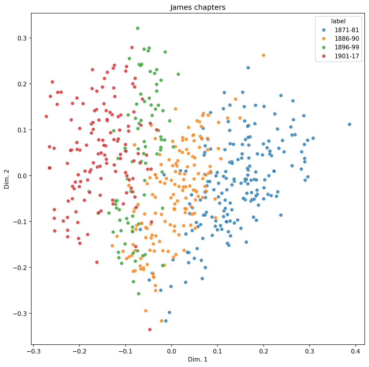
There isn’t perfect separation here. Might some of the overlapping points be mis-classified documents? We run predictions across all documents and re-plot with those.

all_preds = classifier.predict(tfidf)

Where are labels incorrect?

vis_data["incorrect"] = np.where(
    all_preds == vis_data["label_idx"], False, True
)

Re-plot.

plt.figure(figsize = (10, 10))
g = sns.scatterplot(
    x = "x",
    y = "y",
    hue = "label",
    style = "incorrect",
    size = "incorrect",
    sizes = (300, 35),
    palette = "tab10",
    data = vis_data,
    legend = "full"
)
g.set(title = "James chapters", xlabel = "Dim. 1", ylabel = "Dim. 2")
plt.show()

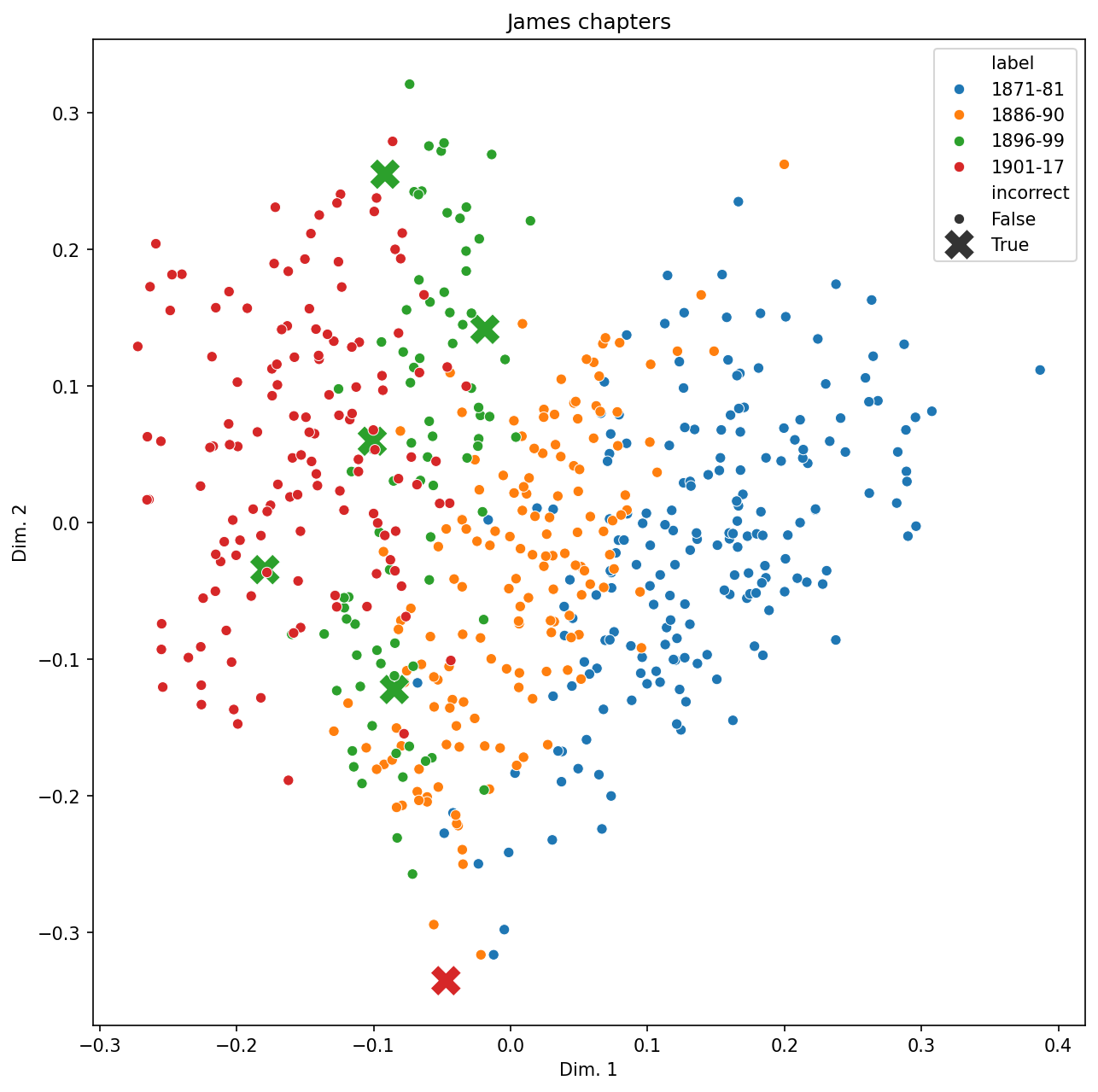
It does indeed seem to be the case that mis-classified documents sit right along the border of two classes. Though keep in mind that dimensionality reduction often results in visual distortions, so looking at data might sometimes be misleading.

Finally, which documents are these?

idx = vis_data[vis_data["incorrect"] == True].index
model_pred = all_preds[idx]
corpus.loc[idx, ["novel", "chapter", "hoover"]].assign(model_pred = model_pred)

	novel	chapter	hoover	model_pred
355	Spoils Poynton	13	2	3
384	What Maisie Knew	20	2	3
400	Awkward Age	5	2	3
422	Awkward Age	27	2	3
424	Awkward Age	29	2	3
562	Ivory Tower	13	3	1