10. Cross Entropy#
This chapter uses toy data to demonstrate how machine learners use cross entropy as a metric for evaluating model fit.
10.1. Preliminaries#
We need the following libraries.
import numpy as np
import pandas as pd
import matplotlib.pyplot as plt
import seaborn as sns
10.2. Data Generation#
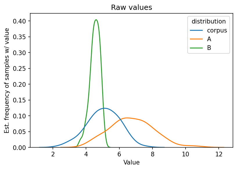
We’re using toy data for this chapter. Below, we randomly sample 100 values
from three distributions with different means (loc) and standard deviations
(scale). We’ll use these values to simulate bigram transitions in text data.
corpus = np.random.normal(loc = 5, scale = 1.0, size = 100)
A = np.random.normal(loc = 6.8, scale = 1.3, size = 100)
B = np.random.normal(loc = 4.5, scale = 0.3, size = 100)
Let’s plot these raw values. First: format into a DataFrame.
df = pd.DataFrame({"corpus": corpus, "A": A, "B": B})
vis = (
    df
    .stack()
    .to_frame("value")
    .reset_index(level = 1)
    .rename(columns = {"level_1": "distribution"})
)
Time to plot.
plt.figure(figsize = (6, 4))
g = sns.kdeplot(x = "value", hue = "distribution", data = vis)
g.set(
    title = "Raw values",
    xlabel = "Value",
    ylabel = "Est. frequency of samples w/ value"
)
plt.show()
10.3. Using Probabilities#
Now, we’ll convert these raw values into probabilities. The above values are continuous, which means they are decimal values. We will “bin” those values so that ones that are close together are counted together in our probability calculation.
def to_probability(samples, n_bins = 10):
    """Discretize samples from a distribution into bins and calculate their
    probabilities.

    Parameters
    ----------
    samples : np.ndarray
        Distribution samples
    n_bins : int
        Number of bins

    Returns
    -------
    probs : np.ndarray
        Bin probabilities
    """
    # Discretize the values into bins
    hist, edges = np.histogram(samples, bins = n_bins, density = True)

    # Calculate the width of each bin. Every sample that falls within this bin
    # is counted in the bin
    width = edges[1] - edges[0]

    # Calculate the probabilities
    probs = hist * width
    probs /= probs.sum()

    return probs
probs = df.apply(to_probability)
For the purposes of demonstration, we’ll label these probabilities as bigrams.
In other words, they represent the likelihood of a bigram sequence. The first,
corpus, represents probabilities from some corpus data. The second two, A
and B, represent the probability of these bigrams according to two language
models.
probs.index = [f"bigram-{i}" for i in range(len(probs))]
probs
| corpus | A | B | |
|---|---|---|---|
| bigram-0 | 0.01 | 0.08 | 0.02 |
| bigram-1 | 0.04 | 0.09 | 0.02 |
| bigram-2 | 0.06 | 0.14 | 0.05 |
| bigram-3 | 0.14 | 0.21 | 0.06 |
| bigram-4 | 0.21 | 0.16 | 0.12 |
| bigram-5 | 0.20 | 0.16 | 0.19 |
| bigram-6 | 0.14 | 0.09 | 0.16 |
| bigram-7 | 0.14 | 0.04 | 0.16 |
| bigram-8 | 0.05 | 0.01 | 0.15 |
| bigram-9 | 0.01 | 0.02 | 0.07 |
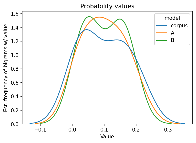
Below, we plot the probabilities. Pay special attention to the shape of the
curves. Does A or B seem to fit corpus better? If so, we could say that
either A or B is a better model for corpus.
First, formatting.
vis = (
    probs
    .stack()
    .to_frame("prob")
    .reset_index(level = 1)
    .rename(columns = {"level_1": "model"})
)
And plot.
plt.figure(figsize = (6, 4))
g = sns.kdeplot(x = "prob", hue = "model", data = vis)
g.set(
    title = "Probability values",
    xlabel = "Value",
    ylabel = "Est. frequency of bigrams w/ value"
)
plt.show()
10.4. Cross Entropy#
But how can we know for sure whether one model is better than another? That’s
where cross entropy comes in. It will tell us how well A or B fit corpus
by providing a loss metric. When language models train, they try to
minimize this metric by updating their weights during each step of the training
process.
def calculate_cross_entropy(Pw, Qw):
    """Calculate the cross-entropy of distribution against another.

    Parameters
    ----------
    Pw : np.ndarray
        True values of the distribution
    Qw : np.ndarray
        Predicted distribution

    Returns
    -------
    cross_entropy : float
        The cross entropy
    """
    # Ensure we have no 0 values
    Qw = np.clip(Qw, 1e-10, 1.0)

    # Unlike in the n-gram modeling chapter, we use natural log in this example
    # because we are not using information elsewhere
    log_Qw = np.log(Qw)
    Sigma = np.sum(Pw * log_Qw)
    cross_entropy = -Sigma

    return cross_entropy
How well do A and B fit corpus?
A_ce = calculate_cross_entropy(probs["corpus"], probs["A"])
B_ce = calculate_cross_entropy(probs["corpus"], probs["B"])
print("A:", A_ce)
print("B:", B_ce)
A: 2.2665247071118846
B: 2.1811955804605505
Which is better, A or B?
choices = ["A", "B"]
idx = np.argmin([A_ce, B_ce])
print(choices[idx])
B