7. Large Language Models: An Introduction#
This chapter introduces large language models (LLMs). We will discuss tokenization strategies, model architecture, the attention mechanism, and dynamic embeddings. Using an example model, we end by dynamically embedding documents to examine how each layer in the model changes documents’ representations.
Data: 59 Emily Dickinson poems collected from the Poetry Foundation
Credits: Portions of this chapter are adapted from the UC Davis DataLab’s Natural Language Processing for Data Science
7.1. Preliminaries#
We need the following libraries:
import torch
import torch.nn as nn
import torch.nn.functional as F
import numpy as np
import pandas as pd
from transformers import AutoTokenizer, AutoModel
from sklearn.metrics.pairwise import cosine_similarity
import circuitsvis as cv
import matplotlib.pyplot as plt
import seaborn as sns
Later, we will work with the Emily Dickinson poems we’ve already seen.
poems = pd.read_parquet("data/datasets/dickinson_poems.parquet")
7.1.1. Using a pretrained model#
Training LLMs requires vast amounts of data and computational resources. While these resources are expensive, the very scale of these models contributes to their ability to generalize. Practitioners will therefore use the same model for a variety of tasks. They do this by pretraining a general model to perform a foundational task, usually next-token prediction. Then, once that model is trained, practitioners fine-tune that model for other tasks. The fine-tuned variants benefit from the generalized language representations learned during pretraining but they adapt those representations to more specific contexts and tasks.
The best place to find these pretrained models is Hugging Face. The company hosts thousands of them on its platform, and it also develops various machine learning tools for working with these models. Hugging Face also features fine-tuned models for various tasks, which may work out of the box for your needs. Take a look at the model listing to see all models on the platform. At left you’ll see categories for model types, task types, and more.
7.1.2. Loading a model#
To load a model from Hugging Face, specify the checkpoint you’d like to use. Typically this is just the name of the model.
checkpoint = "google-bert/bert-base-uncased"
The transformers library has different tokenizer and model classes for
different models/architectures and tasks. You can write these out directly, or
use the Auto* classes, which dynamically determine what class you’ll need for
a model and task. Below, we load the base BERT model without specifying a task.
tokenizer = AutoTokenizer.from_pretrained(checkpoint)
bert = AutoModel.from_pretrained(checkpoint)
If you don’t have this model stored on your own computer, it will download
directly from Hugging Face. The default directory for storing Hugging Face data
is ~/.cache/hugggingface. Set a HF_HOME environment variable from the
command line do direct downloads to a different location on your computer.
export HF_HOME=/path/to/another/directory
7.2. Subword Tokenization#
You may have noticed that we initialized a tokenizer and model from the same checkpoint. This is important: LLMs depend on specific tokenizers, which are themselves trained on corpus data before their corresponding models even see that data. But why do tokenizers need to be trained in the first place?
The answer has to do with the highly general nature of LLMs. These models are trained on huge corpora, which means they must represent millions of different pieces of text. Model vocabularies would quickly balloon to a huge size if they represented all unique tokens, however, and at any rate this would be both inefficient and a waste of resources, since some tokens are extremely rare. In traditional tokenization and model building, you’d set a cutoff below which rare tokens could be ignored, but LLMs need all text. That means they need to represent every token in a corpus—without storing representations for every token in a corpus.
Model developers square this circle by using pieces of words, or subwords, to represent other tokens. That way, a model can literally spell out any text sequence it needs to build without having representations for every unique token in its training corpus. (This also means LLMs can handle text they’ve never seen before.) Setting the cutoff for which tokens should be represented in full and which are best represented by subwords requires training a tokenizer to learn the token distribution in a corpus, build subwords, and determine said cutoff.
With subword tokenization, the following phrase:
large language models use subword tokenization
…becomes:
large language models use sub ##word token ##ization
See the hashes? This tokenizer prepends them to its subwords.
7.2.1. Input IDs#
The actual output of transformers tokenizer has a few parts. We use the
following sentence as an example:
sentence = "Then I tried to find some way of embracing my mother's ghost."
Send this to the tokenizer, setting the return type to PyTorch tensors. We also return the attention mask.
inputs = tokenizer(
    sentence, return_tensors = "pt", return_attention_mask = True
)
Input IDs are the unique identifiers for every token in the input text. These are what the model actually looks at.
inputs["input_ids"]
tensor([[  101,  2059,  1045,  2699,  2000,  2424,  2070,  2126,  1997, 23581,
          2026,  2388,  1005,  1055,  5745,  1012,   102]])
Use the .decode() method to transform an ID (or sequences of ids) back to
text.
tokenizer.decode(5745)
'ghost'
The tokenizer has entries for punctuation:
tokenizer.decode([1005, 1012])
"'."
Whitespace tokens are often removed, however:
ws = tokenizer(" \t\n")
ws["input_ids"]
[101, 102]
But if that’s the case, what are those two IDs? These are two special tokens that BERT uses for a few different tasks.
tokenizer.decode([101, 102])
'[CLS] [SEP]'
[CLS] is prepended to every input sequence. It marks the start of a sequence,
and it also serves as a “summarization” token for sequences, a kind of
aggregate representation of model outputs. When you train a model for
classification tasks, the model uses [CLS] to decide how to categorize a
sequence.
[SEP] is appended to every input sequence. It marks the end of a sequence,
and it is used to separate input pairs for tasks like sentence similarity,
question answering, and summarization. When training, a model looks to [SEP]
to distinguish which parts of the input correspond to task components.
7.2.2. Token type IDs#
Some models don’t need anything more than [CLS] and [SEP] to make the above
distinctions. But other models also incorporate token type IDs to further
distinguish individual pieces of input. These IDs are binary values that tell
the model which parts of the input belong to what components in the task.
Our sentence makes no distinction:
inputs["token_type_ids"]
tensor([[0, 0, 0, 0, 0, 0, 0, 0, 0, 0, 0, 0, 0, 0, 0, 0, 0]])
But a pair of sentences would:
question = "What did I do then?"
with_token_types = tokenizer(question, sentence)
with_token_types["token_type_ids"]
[0, 0, 0, 0, 0, 0, 0, 0, 1, 1, 1, 1, 1, 1, 1, 1, 1, 1, 1, 1, 1, 1, 1, 1]
7.2.3. Attention mask#
A final output, attention mask, tells the model what part of the input it should use when it processes the sequence.
inputs["attention_mask"]
tensor([[1, 1, 1, 1, 1, 1, 1, 1, 1, 1, 1, 1, 1, 1, 1, 1, 1]])
7.2.4. Padding and truncation#
It may seem like a redundancy to add an attention mask, but tokenizers often pad input sequences. While Transformer models can process sequences in parallel, which massively speeds up their run time, each sequence in a batch needs to be the same length. Texts, however, are rarely the same length, hence the padding.
two_sequence_inputs = tokenizer(
    [question, sentence],
    return_tensors = "pt",
    return_attention_mask = True,
    padding = "longest"
)
two_sequence_inputs["input_ids"]
tensor([[  101,  2054,  2106,  1045,  2079,  2059,  1029,   102,     0,     0,
             0,     0,     0,     0,     0,     0,     0],
        [  101,  2059,  1045,  2699,  2000,  2424,  2070,  2126,  1997, 23581,
          2026,  2388,  1005,  1055,  5745,  1012,   102]])
Token ID 0 is the [PAD] token.
tokenizer.decode(0)
'[PAD]'
And here are the attention masks:
two_sequence_inputs["attention_mask"]
tensor([[1, 1, 1, 1, 1, 1, 1, 1, 0, 0, 0, 0, 0, 0, 0, 0, 0],
        [1, 1, 1, 1, 1, 1, 1, 1, 1, 1, 1, 1, 1, 1, 1, 1, 1]])
There are a few different strategies for padding. Above, we had the tokenizer
pad to the longest sequence in the input. But usually it’s best to set it to
max_length:
two_sequence_inputs = tokenizer(
    [question, sentence],
    return_tensors = "pt",
    return_attention_mask = True,
    padding = "max_length"
)
two_sequence_inputs["input_ids"][0]
tensor([ 101, 2054, 2106, 1045, 2079, 2059, 1029,  102,    0,    0,    0,    0,
           0,    0,    0,    0,    0,    0,    0,    0,    0,    0,    0,    0,
           0,    0,    0,    0,    0,    0,    0,    0,    0,    0,    0,    0,
           0,    0,    0,    0,    0,    0,    0,    0,    0,    0,    0,    0,
           0,    0,    0,    0,    0,    0,    0,    0,    0,    0,    0,    0,
           0,    0,    0,    0,    0,    0,    0,    0,    0,    0,    0,    0,
           0,    0,    0,    0,    0,    0,    0,    0,    0,    0,    0,    0,
           0,    0,    0,    0,    0,    0,    0,    0,    0,    0,    0,    0,
           0,    0,    0,    0,    0,    0,    0,    0,    0,    0,    0,    0,
           0,    0,    0,    0,    0,    0,    0,    0,    0,    0,    0,    0,
           0,    0,    0,    0,    0,    0,    0,    0,    0,    0,    0,    0,
           0,    0,    0,    0,    0,    0,    0,    0,    0,    0,    0,    0,
           0,    0,    0,    0,    0,    0,    0,    0,    0,    0,    0,    0,
           0,    0,    0,    0,    0,    0,    0,    0,    0,    0,    0,    0,
           0,    0,    0,    0,    0,    0,    0,    0,    0,    0,    0,    0,
           0,    0,    0,    0,    0,    0,    0,    0,    0,    0,    0,    0,
           0,    0,    0,    0,    0,    0,    0,    0,    0,    0,    0,    0,
           0,    0,    0,    0,    0,    0,    0,    0,    0,    0,    0,    0,
           0,    0,    0,    0,    0,    0,    0,    0,    0,    0,    0,    0,
           0,    0,    0,    0,    0,    0,    0,    0,    0,    0,    0,    0,
           0,    0,    0,    0,    0,    0,    0,    0,    0,    0,    0,    0,
           0,    0,    0,    0,    0,    0,    0,    0,    0,    0,    0,    0,
           0,    0,    0,    0,    0,    0,    0,    0,    0,    0,    0,    0,
           0,    0,    0,    0,    0,    0,    0,    0,    0,    0,    0,    0,
           0,    0,    0,    0,    0,    0,    0,    0,    0,    0,    0,    0,
           0,    0,    0,    0,    0,    0,    0,    0,    0,    0,    0,    0,
           0,    0,    0,    0,    0,    0,    0,    0,    0,    0,    0,    0,
           0,    0,    0,    0,    0,    0,    0,    0,    0,    0,    0,    0,
           0,    0,    0,    0,    0,    0,    0,    0,    0,    0,    0,    0,
           0,    0,    0,    0,    0,    0,    0,    0,    0,    0,    0,    0,
           0,    0,    0,    0,    0,    0,    0,    0,    0,    0,    0,    0,
           0,    0,    0,    0,    0,    0,    0,    0,    0,    0,    0,    0,
           0,    0,    0,    0,    0,    0,    0,    0,    0,    0,    0,    0,
           0,    0,    0,    0,    0,    0,    0,    0,    0,    0,    0,    0,
           0,    0,    0,    0,    0,    0,    0,    0,    0,    0,    0,    0,
           0,    0,    0,    0,    0,    0,    0,    0,    0,    0,    0,    0,
           0,    0,    0,    0,    0,    0,    0,    0,    0,    0,    0,    0,
           0,    0,    0,    0,    0,    0,    0,    0,    0,    0,    0,    0,
           0,    0,    0,    0,    0,    0,    0,    0,    0,    0,    0,    0,
           0,    0,    0,    0,    0,    0,    0,    0,    0,    0,    0,    0,
           0,    0,    0,    0,    0,    0,    0,    0,    0,    0,    0,    0,
           0,    0,    0,    0,    0,    0,    0,    0,    0,    0,    0,    0,
           0,    0,    0,    0,    0,    0,    0,    0])
This will pad the text out to the maximum number of tokens the model can process at once. This number is known as the context window.
print("Context window size:", tokenizer.model_max_length)
Context window size: 512
Warning
Not all tokenizers have this information stored in their configuration. You should always check whether this is the case before you use a tokenizer. If it doesn’t have this information, take a look at the model documentation.
If your input exceeds the number above, you will need to truncate it, otherwise the model may not process input properly.
too_long = "a " * 10_000
too_long_inputs = tokenizer(
    too_long, return_tensors = "pt", return_attention_mask = True
)
Token indices sequence length is longer than the specified maximum sequence length for this model (10002 > 512). Running this sequence through the model will result in indexing errors
Set truncation to True to avoid this problem.
too_long_inputs = tokenizer(
    too_long,
    return_tensors = "pt",
    return_attention_mask = True,
    padding = "max_length",
    truncation = True
)
What if you have long texts, like novels? You’ll need to make some decisions. You could, for example, look for a model with a bigger context window; several of the newest LLMs can process novel-length documents now. Or, you might strategically chunk your text. Perhaps you’re only interested in dialogue, or maybe paragraph-length descriptions. You could preprocess your texts to create chunks of this kind, ensure they do not exceed your context window size, and then send them to the model.
Regardless of what strategy you use, it will take iterative tries to settle on a final tokenization workflow.
7.3. Components of the Transformer#
Before we process our tokens, let’s overview what happens when we send input to the model. Here are all the components of the model:
bert
BertModel(
  (embeddings): BertEmbeddings(
    (word_embeddings): Embedding(30522, 768, padding_idx=0)
    (position_embeddings): Embedding(512, 768)
    (token_type_embeddings): Embedding(2, 768)
    (LayerNorm): LayerNorm((768,), eps=1e-12, elementwise_affine=True)
    (dropout): Dropout(p=0.1, inplace=False)
  )
  (encoder): BertEncoder(
    (layer): ModuleList(
      (0-11): 12 x BertLayer(
        (attention): BertAttention(
          (self): BertSdpaSelfAttention(
            (query): Linear(in_features=768, out_features=768, bias=True)
            (key): Linear(in_features=768, out_features=768, bias=True)
            (value): Linear(in_features=768, out_features=768, bias=True)
            (dropout): Dropout(p=0.1, inplace=False)
          )
          (output): BertSelfOutput(
            (dense): Linear(in_features=768, out_features=768, bias=True)
            (LayerNorm): LayerNorm((768,), eps=1e-12, elementwise_affine=True)
            (dropout): Dropout(p=0.1, inplace=False)
          )
        )
        (intermediate): BertIntermediate(
          (dense): Linear(in_features=768, out_features=3072, bias=True)
          (intermediate_act_fn): GELUActivation()
        )
        (output): BertOutput(
          (dense): Linear(in_features=3072, out_features=768, bias=True)
          (LayerNorm): LayerNorm((768,), eps=1e-12, elementwise_affine=True)
          (dropout): Dropout(p=0.1, inplace=False)
        )
      )
    )
  )
  (pooler): BertPooler(
    (dense): Linear(in_features=768, out_features=768, bias=True)
    (activation): Tanh()
  )
)
These pieces are divided up into an embeddings portion and an encoder portion. Both are accessible:
bert.embeddings
BertEmbeddings(
  (word_embeddings): Embedding(30522, 768, padding_idx=0)
  (position_embeddings): Embedding(512, 768)
  (token_type_embeddings): Embedding(2, 768)
  (LayerNorm): LayerNorm((768,), eps=1e-12, elementwise_affine=True)
  (dropout): Dropout(p=0.1, inplace=False)
)
…and
bert.encoder
BertEncoder(
  (layer): ModuleList(
    (0-11): 12 x BertLayer(
      (attention): BertAttention(
        (self): BertSdpaSelfAttention(
          (query): Linear(in_features=768, out_features=768, bias=True)
          (key): Linear(in_features=768, out_features=768, bias=True)
          (value): Linear(in_features=768, out_features=768, bias=True)
          (dropout): Dropout(p=0.1, inplace=False)
        )
        (output): BertSelfOutput(
          (dense): Linear(in_features=768, out_features=768, bias=True)
          (LayerNorm): LayerNorm((768,), eps=1e-12, elementwise_affine=True)
          (dropout): Dropout(p=0.1, inplace=False)
        )
      )
      (intermediate): BertIntermediate(
        (dense): Linear(in_features=768, out_features=3072, bias=True)
        (intermediate_act_fn): GELUActivation()
      )
      (output): BertOutput(
        (dense): Linear(in_features=3072, out_features=768, bias=True)
        (LayerNorm): LayerNorm((768,), eps=1e-12, elementwise_affine=True)
        (dropout): Dropout(p=0.1, inplace=False)
      )
    )
  )
)
7.3.1. Input embeddings#
The first layer in a LLM is typically the word embeddings matrix. These embeddings are the starting values for every token in the model’s vocabulary and have not been encoded with any contextual information. Think of them like model defaults.
embeddings = bert.embeddings.word_embeddings(inputs["input_ids"])
Note the shape of these embeddings:
embeddings.shape
torch.Size([1, 17, 768])
Models assume you are working with batches, so the first number corresponds to the number of sequences in the batch. The second number corresponds to tokens and the third to each feature in the vectors that represent those tokens.
For the purposes of demonstration, we drop the batch layer with .squeeze().
embeddings = embeddings.squeeze(0)
7.3.2. Other default embeddings#
BERT-style models (like the one here) also have positional embeddings, which are learned during training. Each index in the context window has a positional embedding vector that corresponds with it.
bert.embeddings.position_embeddings.weight
There is also a embedding matrix for token type embeddings. These differentiate input segments.
bert.embeddings.token_type_embeddings
7.3.3. Attention#
If you look back to the encoder part of the model, you’ll see that first component in a layer block is an attention mechanism. This mechanism enables the model to draw many-to-many relationships between tokens. During training, attention helps the model form strong (or weak) relationships between certain tokens, which in turn allows it to focus on different parts of input sequences dynamically. When fed an input sequence, the model learns to privilege relationships between certain parts of the input over others, and in doing so it captures complex patterns, local contexts, and long-range dependencies among the tokens.
You will often see different forms of attention described in the context of Transformers. We will walk through the three main ones. At core, however, attention is expressed as the following:
Where:
\(Q\), \(K\), and \(V\) are query, key, and value matrices, which correspond to all tokens in an input sequence
\(d_k\) is the dimensionality of the key matrix
\(softmax\) expresses result as a probability distribution of possible outcomes
The following function implements this equation.
def scaled_dot_product_attention(Q, K, V, mask = None):
    """Calculate scaled dot-product attention.

    Parameters
    ----------
    Q, K, V : torch.Tensor
        Query, key, and value matrices
    mask : None or torch.Tensor
        A triangular masking matrix

    Returns
    -------
    weighted : torch.Tensor
        Word embeddings weighted by attention
    """
    # Perform matrix multiplication to query the keys (dot product of i-th and
    # j-th scores of `Q` and `K`). Note the transpose of `K`
    scores = torch.matmul(Q, K.transpose(-2, -1))

    # Normalize the scores with the square root of the dimensionality of `K`.
    # This reduces the magnitude of the scores, thereby preventing them from
    # becoming too large (which would in turn create vanishingly small
    # gradients during back propagation)
    d_k = K.size(-1)
    scores = scores / torch.sqrt(torch.tensor(d_k, dtype = torch.float32))

    # Are we masking tokens to the right?
    if mask is not None:
        scores = scores.masked_fill(mask == 0, float("-inf"))

    # Compute softmax to convert attention scores into probabilities. Every row
    # in `probs` is a probability distribution across every token in the model
    probs = F.softmax(scores, dim = -1)

    # Perform a final matrix multiplication between `probs` and `V`. Here,
    # `probs` acts as a set of weights by which to modify the original
    # embeddings. Matrix multiplication will aggregate all values in `V`,
    # producing a weighted sum
    weighted = torch.matmul(probs, V)

    return weighted
Self-attention means that each token in an input sequence is compared with every other token. This enables the model to capture relationships across the entire input sequence.
Q = K = V = embeddings
attention_scores = scaled_dot_product_attention(Q, K, V)
The above calculates attention in a bi-directional manner, meaning tokens to the left and right of a token are taken into account. This is what models like BERT use. Calculating attention in a uni-directional manner, which is what models like GPT use, requires masking out tokens to the right.
mask = torch.tril(torch.ones(Q.size(-2), K.size(-2)), diagonal = 1).bool()
attention_scores = scaled_dot_product_attention(Q, K, V, mask)
You will often see the above referred to as causal-attention. Note however that it is still technically self-attention.
Cross-attention takes an external set of embeddings for the query matrix. In translation models, for example, these are embeddings for a target language into which a model is transforming sentences from a source language. We simulate the external embeddings with random ones below.
K_source = V_source = embeddings
Q_target = torch.rand_like(embeddings)
attention_scores = scaled_dot_product_attention(Q_target, K_source, V_source)
Multi-head attention involves using multiple attention mechanisms, or heads, in parallel, which are then concatenated together when they are passed elsewhere in the network. During training, each head learns to focus on different kinds of relationships in the text data.
This is what a head split looks like:
n_heads = 12
n_tokens, n_dim = embeddings.shape
head_dim = n_dim // n_heads
heads = embeddings.view(n_tokens, n_heads, head_dim).transpose(0, 1)
Then, you perform attention for each one, concatenate them all, and reshape.
head_outputs = []
for i in range(n_heads):
    Q, K, V = heads[i]
    scores = scaled_dot_product_attention(Q, K, V)
    head_outputs.append(scores)

attention_scores = torch.cat(head_outputs, dim = -1).view(n_tokens, n_dim)
All of the above, however, is implemented in PyTorch. First, we initialize the layer.
attention_layer = nn.MultiHeadAttention(embed_dim = 768, num_heads = 12)
Then we build the key, query, and value matrices. With those built, we run them through the layer.
Q = K = V = embeddings.transpose(0, 1)
attention_scores, _ = attention_layer(Q, K, V)
attention_scores = attention_scores.transpose(0, 1)
7.3.4. Linear transform#
Once attention scores are computed, the model passes them through a linear layer. You will also see this called a “fully connected” layer—that is, it connects every input neuron to every output neuron. This layer maps an input matrix to an output matrix via learnable parameters: a weight matrix and a bias vector.
We express the transformation as follows:
Where, for the resultant matrix \(y\):
\(W\) is a weight matrix with dimensions \((m, p)\), where \(m\) is the number of input features and \(p\) is the number of output features
\(x\) is an input matrix with dimensions \((n, m)\), where \(n\) is the batch size
\(b\) is a bias vector with dimensions \(p\)
Every value in \(W\) determines how much each input feature contributes to the output. This emphasizes the importance (or lack of importance) of features for a training task. Additionally, a linear transformation projects attention scores into a new feature space, which helps to summarize relationships in the input data and capture complex patterns.
linear_layer = nn.Linear(in_features = 768, out_features = 3072, bias = True)
transformed = linear_layer(attention_scores)
7.3.5. Normalization and dropout#
With the new projection created, the model then applies normalization and dropout.
Normalization standardizes inputs. This helps to stabilize the model training by constraining values to a smaller range. It also speeds up computations.
norm_layer = nn.BatchNorm1d(num_features = 768)
normed = norm_layer(transformed)
The dropout layer randomly zeros-out a set percentage of values in its input matrix. This combats overfitting by preventing the model from becoming too reliant on any single dimension.
dropout_layer = nn.Dropout(p = 0.1)
dropped = dropout_layer(normalized)
7.3.6. Activation layer#
Finally, after the model runs through blocks of attention, linear transformation, and normalization/dropout, it passes the data through an activation layer. This layer introduces non-linearity in the model, which in turn allows it to learn more complex patterns that cannot be approximated through simple, linear relationships. You can think of linear layers as filters of a sort: they use specially designed cutoffs to determine how input values are transformed into outputs.
There are several different kinds of activation functions. We’ll demonstrate a few below. First, we create a set of linear input values \([-5, 5]\) and initialize a dictionary of our functions.
x = torch.linspace(-5, 5, 100, dtype = torch.float32)
activation_functions = {
    "original": lambda data: data,
    "tanh": nn.Tanh(),
    "sigmoid": nn.Sigmoid(),
    "ReLU": nn.ReLU(),
    "GELU": nn.GELU()
}
We put our values through every activation function and format the results as a DataFrame.
activated = []
for name, func in activation_functions.items():
    y = func(x).numpy()
    activated.extend([(name, xi, yi) for xi, yi in zip(x.numpy(), y)])

activated = pd.DataFrame(activated, columns = ["activation", "x", "y"])
Now plot.
plt.figure(figsize = (4, 4))
g = sns.lineplot(
    x = "x",
    y = "y",
    hue = "activation",
    style = "activation",
    dashes = [(2, 2), "", "", "", ""],
    alpha = 0.8,
    data = activated
)
g.set(
    title = "Activation Functions",
    xlabel = "Input values",
    ylabel = "Output values",
)
plt.legend(loc = "upper left", bbox_to_anchor = (1, 1))
plt.grid(True)
plt.show()
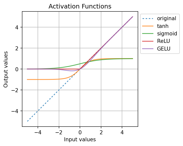
GELU, or Gaussian Error Linear Unit, is a popular activation function for Transformers.
activation_layer = nn.GELU()
activated = activation_layer(dropped)
7.4. Running the Model#
This is a lot of information and a lot of steps. Luckily, all of the above will
happen in a single call. But first, let’s move our model to a device (like a
GPU, represented as 0 below). The transformers library is pretty good at
doing this for us, but we can always do so explicitly:
device = 0 if torch.cuda.is_available() else "cpu"
bert.to(device)

print(f"Moved model to {device}")
Moved model to cpu
Tip
You can also set the model device when initializing it.
model = AutoModel.from_pretrained(checkpoint, device = device)
Time to process the inputs. First, put the model in evaluation mode. This disables dropout, which can make outputs inconsistent (e.g. non-deterministic).
bert.eval()
BertModel(
  (embeddings): BertEmbeddings(
    (word_embeddings): Embedding(30522, 768, padding_idx=0)
    (position_embeddings): Embedding(512, 768)
    (token_type_embeddings): Embedding(2, 768)
    (LayerNorm): LayerNorm((768,), eps=1e-12, elementwise_affine=True)
    (dropout): Dropout(p=0.1, inplace=False)
  )
  (encoder): BertEncoder(
    (layer): ModuleList(
      (0-11): 12 x BertLayer(
        (attention): BertAttention(
          (self): BertSdpaSelfAttention(
            (query): Linear(in_features=768, out_features=768, bias=True)
            (key): Linear(in_features=768, out_features=768, bias=True)
            (value): Linear(in_features=768, out_features=768, bias=True)
            (dropout): Dropout(p=0.1, inplace=False)
          )
          (output): BertSelfOutput(
            (dense): Linear(in_features=768, out_features=768, bias=True)
            (LayerNorm): LayerNorm((768,), eps=1e-12, elementwise_affine=True)
            (dropout): Dropout(p=0.1, inplace=False)
          )
        )
        (intermediate): BertIntermediate(
          (dense): Linear(in_features=768, out_features=3072, bias=True)
          (intermediate_act_fn): GELUActivation()
        )
        (output): BertOutput(
          (dense): Linear(in_features=3072, out_features=768, bias=True)
          (LayerNorm): LayerNorm((768,), eps=1e-12, elementwise_affine=True)
          (dropout): Dropout(p=0.1, inplace=False)
        )
      )
    )
  )
  (pooler): BertPooler(
    (dense): Linear(in_features=768, out_features=768, bias=True)
    (activation): Tanh()
  )
)
Then, wrap the process in a context manager. This context manager will keep the model from collecting gradients when it processes. Unless you are training a model or trying understand model internals, there’s no need for gradients. With the context manager built, send the inputs to the model.
with torch.no_grad():
    outputs = bert(**inputs, output_hidden_states = True)
7.4.1. Model outputs#
There are several components in this output:
outputs
BaseModelOutputWithPoolingAndCrossAttentions(last_hidden_state=tensor([[[-0.1813, -0.1627, -0.2402,  ..., -0.1174,  0.2389,  0.5933],
         [-0.1219,  0.2374, -0.8745,  ...,  0.3379,  0.4232, -0.2547],
         [ 0.3440,  0.2197, -0.0133,  ..., -0.1566,  0.2564,  0.2016],
         ...,
         [ 0.5548, -0.4396,  0.7075,  ...,  0.1718, -0.1337,  0.4442],
         [ 0.5042,  0.1461, -0.2642,  ...,  0.0728, -0.4193, -0.3139],
         [ 0.4306,  0.1996, -0.0055,  ...,  0.1924, -0.5685, -0.3190]]]), pooler_output=tensor([[-9.0215e-01, -3.6355e-01, -8.6364e-01,  6.3150e-01,  5.2959e-01,
         -2.3988e-01,  7.8954e-01,  1.9048e-01, -7.7929e-01, -9.9996e-01,
         -1.1218e-01,  9.3984e-01,  9.7191e-01,  2.6334e-01,  8.9467e-01,
         -6.9052e-01, -3.4147e-01, -5.5349e-01,  2.6398e-01, -4.4079e-01,
          6.8211e-01,  9.9988e-01,  6.3717e-02,  1.4847e-01,  4.0085e-01,
          9.8006e-01, -5.9317e-01,  8.9493e-01,  9.5012e-01,  6.7092e-01,
         -5.0414e-01,  1.7098e-01, -9.8875e-01,  9.4529e-03, -7.9112e-01,
         -9.8928e-01,  1.5902e-01, -6.4964e-01,  1.5020e-01,  1.5166e-01,
         -9.0359e-01,  2.1367e-01,  9.9995e-01, -4.1530e-01,  4.3635e-01,
         -1.1558e-01, -1.0000e+00,  2.2613e-01, -8.9463e-01,  8.5809e-01,
          8.1223e-01,  9.0436e-01,  8.7882e-02,  4.7012e-01,  4.0199e-01,
         -2.3712e-01, -1.9334e-01,  4.6882e-04, -2.2115e-01, -5.5566e-01,
         -5.7362e-01,  3.4552e-01, -7.4646e-01, -8.7389e-01,  8.9060e-01,
          6.6513e-01, -2.7116e-02, -1.4315e-01, -4.6456e-02, -1.1431e-01,
          8.5752e-01,  4.0294e-02,  1.1696e-02, -8.3643e-01,  4.3631e-01,
          1.6847e-01, -5.5569e-01,  1.0000e+00, -4.2451e-01, -9.7485e-01,
          7.4691e-01,  6.4409e-01,  4.5656e-01,  7.3656e-02,  1.3891e-01,
         -1.0000e+00,  6.1069e-01,  8.5232e-02, -9.8454e-01,  5.9957e-02,
          5.2395e-01, -2.2201e-01,  1.2185e-01,  5.0690e-01, -3.0269e-01,
         -4.4167e-01, -1.1198e-01, -7.8108e-01, -9.9268e-02, -3.5597e-01,
         -1.5475e-02,  6.0668e-02, -2.7171e-01, -1.8928e-01,  2.8009e-01,
         -4.4744e-01, -6.4973e-01,  2.8635e-01,  3.2423e-03,  5.7549e-01,
          3.8756e-01, -2.1564e-01,  2.9823e-01, -9.4773e-01,  5.1873e-01,
         -2.5598e-01, -9.8738e-01, -5.5347e-01, -9.8613e-01,  6.5802e-01,
         -1.9799e-01, -2.3325e-01,  9.4350e-01,  7.4329e-02,  2.8480e-01,
          1.1823e-01, -9.1459e-01, -1.0000e+00, -7.1362e-01, -3.3832e-01,
         -1.5427e-02, -2.2573e-01, -9.7104e-01, -9.5031e-01,  5.0464e-01,
          9.3296e-01,  1.1413e-01,  9.9982e-01, -1.4094e-01,  9.2251e-01,
         -1.1937e-02, -5.9505e-01,  6.0277e-01, -3.5788e-01,  6.4097e-01,
         -5.7841e-02, -2.5286e-01,  2.0187e-01, -2.5656e-01,  4.5353e-01,
         -6.9229e-01, -3.8542e-03, -6.3896e-01, -8.9819e-01, -2.3500e-01,
          9.3484e-01, -4.6395e-01, -8.6960e-01, -3.4996e-02, -7.0627e-02,
         -3.8399e-01,  7.3087e-01,  7.5051e-01,  2.9726e-01, -3.3074e-01,
          3.7799e-01, -1.4909e-01,  4.0023e-01, -7.6468e-01, -4.4099e-02,
          4.0490e-01, -2.2321e-01, -6.1502e-01, -9.8328e-01, -2.5075e-01,
          5.6157e-01,  9.8075e-01,  6.5358e-01,  5.6203e-02,  7.9783e-01,
         -1.8338e-01,  7.3604e-01, -9.2419e-01,  9.7970e-01,  2.9938e-02,
          5.1264e-02, -8.8993e-04,  5.2048e-01, -8.5517e-01, -2.0054e-01,
          7.7441e-01, -6.9283e-01, -8.3609e-01, -9.7109e-04, -3.6640e-01,
         -2.3179e-01, -6.8952e-01,  5.6256e-01, -1.9093e-01, -1.7197e-01,
          1.5008e-01,  9.0820e-01,  9.2894e-01,  7.8880e-01,  1.3647e-01,
          6.8747e-01, -8.5234e-01, -3.4889e-01,  1.4948e-02,  7.0052e-02,
          8.3297e-02,  9.9249e-01, -5.5713e-01,  1.2017e-02, -9.3871e-01,
         -9.8170e-01, -2.3915e-01, -8.9892e-01, -4.3212e-02, -5.4737e-01,
          5.8934e-01, -2.9702e-01,  3.1357e-01,  3.1863e-01, -9.4778e-01,
         -6.9678e-01,  3.0899e-01, -4.9348e-01,  3.4331e-01, -3.1521e-01,
          9.4813e-01,  8.7397e-01, -4.9162e-01,  4.0090e-01,  9.2305e-01,
         -8.6857e-01, -7.5446e-01,  6.5415e-01, -2.4450e-01,  8.2804e-01,
         -5.3416e-01,  9.8093e-01,  8.6154e-01,  8.7709e-01, -8.8134e-01,
         -5.8875e-01, -7.7638e-01, -4.9128e-01,  6.3842e-02, -3.1175e-01,
          8.1792e-01,  5.7528e-01,  3.3582e-01,  6.7806e-01, -5.1993e-01,
          9.9162e-01, -9.6824e-01, -9.4774e-01, -5.3149e-01,  2.6096e-02,
         -9.8804e-01,  8.2734e-01,  1.6417e-01,  3.2679e-01, -4.0681e-01,
         -4.9522e-01, -9.5393e-01,  7.7904e-01, -1.4957e-03,  9.6117e-01,
         -2.7639e-01, -8.6071e-01, -6.4372e-01, -9.0329e-01, -2.5810e-01,
         -1.1203e-01, -1.1593e-01, -2.3476e-01, -9.4845e-01,  3.6636e-01,
          5.2653e-01,  5.2235e-01, -6.2701e-01,  9.9611e-01,  1.0000e+00,
          9.7235e-01,  8.7527e-01,  8.2946e-01, -9.9941e-01, -6.6086e-01,
          9.9998e-01, -9.8423e-01, -1.0000e+00, -9.1387e-01, -6.1058e-01,
          9.1625e-02, -1.0000e+00, -1.6898e-01,  1.8335e-01, -9.1385e-01,
          6.8013e-01,  9.7530e-01,  9.8308e-01, -1.0000e+00,  8.5240e-01,
          9.2787e-01, -5.7181e-01,  9.1319e-01, -3.5524e-01,  9.6975e-01,
          3.2755e-01,  5.3928e-01, -2.5199e-02,  2.4171e-01, -8.6792e-01,
         -7.3762e-01, -3.5711e-01, -7.3350e-01,  9.9496e-01,  9.6279e-02,
         -7.7655e-01, -8.4988e-01,  6.1927e-01,  2.1021e-03, -3.2598e-01,
         -9.5913e-01, -1.0941e-01,  5.3905e-01,  7.7692e-01,  2.0210e-01,
          1.3288e-01, -5.2597e-01,  1.3350e-01, -3.0387e-01,  3.1106e-02,
          6.0131e-01, -9.2876e-01, -4.0126e-01,  9.3838e-02, -9.1770e-02,
         -2.1734e-01, -9.5718e-01,  9.5094e-01, -2.4999e-01,  8.7258e-01,
          1.0000e+00,  4.4012e-01, -8.2275e-01,  5.4966e-01,  1.5370e-01,
          2.0310e-01,  1.0000e+00,  7.8576e-01, -9.7345e-01, -5.6520e-01,
          5.5103e-01, -4.8463e-01, -6.1582e-01,  9.9890e-01, -1.2441e-01,
         -5.9766e-01, -4.3516e-01,  9.7372e-01, -9.8673e-01,  9.8594e-01,
         -8.5766e-01, -9.6840e-01,  9.5956e-01,  9.2108e-01, -6.8813e-01,
         -7.0525e-01,  3.6422e-02, -4.2375e-01,  1.7284e-01, -9.3253e-01,
          7.1364e-01,  3.9647e-01, -9.4511e-02,  8.9084e-01, -5.6835e-01,
         -5.2339e-01,  1.4913e-01, -6.5024e-01, -1.9193e-01,  9.0409e-01,
          4.0446e-01, -7.4188e-02, -5.9329e-02, -1.0553e-01, -8.4495e-01,
         -9.6772e-01,  6.0419e-01,  1.0000e+00,  1.2257e-02,  7.9661e-01,
         -2.5697e-01,  7.9121e-02, -2.7145e-01,  3.9955e-01,  3.5015e-01,
         -1.9779e-01, -8.1081e-01,  6.1581e-01, -9.3205e-01, -9.8435e-01,
          5.6242e-01,  2.5414e-02, -1.9855e-01,  9.9998e-01,  3.9147e-01,
          3.8831e-02,  3.6355e-01,  9.7193e-01, -1.5554e-01,  3.0005e-01,
          7.3116e-01,  9.7749e-01, -1.4626e-01,  5.5644e-01,  7.9268e-01,
         -8.0457e-01, -2.1986e-01, -5.8049e-01, -1.1498e-01, -9.2331e-01,
          2.5465e-01, -9.5982e-01,  9.4562e-01,  9.3056e-01,  2.6739e-01,
         -4.9384e-04,  5.2062e-01,  1.0000e+00, -8.0677e-01,  3.9905e-01,
          2.6592e-01,  5.3715e-01, -9.9927e-01, -7.9586e-01, -3.2750e-01,
         -5.8726e-02, -6.6198e-01, -2.9297e-01,  1.0346e-01, -9.6175e-01,
          5.6368e-01,  5.5213e-01, -9.7025e-01, -9.8716e-01, -3.4926e-01,
          7.4946e-01,  6.1641e-02, -9.7373e-01, -7.1220e-01, -3.7798e-01,
          5.8977e-01, -1.0241e-01, -9.3295e-01,  2.2246e-02, -1.3604e-01,
          5.2007e-01, -8.4998e-02,  5.1492e-01,  7.3342e-01,  8.4501e-01,
         -5.2785e-01, -2.8822e-01,  4.6259e-02, -6.9614e-01,  8.7093e-01,
         -7.8254e-01, -8.6091e-01, -4.9410e-03,  1.0000e+00, -4.8026e-01,
          8.4091e-01,  6.7065e-01,  7.7482e-01, -1.2159e-01,  1.1097e-01,
          7.9307e-01,  2.5259e-01, -4.3484e-01, -7.9768e-01, -5.9233e-03,
         -2.7596e-01,  6.4743e-01,  4.9924e-01,  4.2030e-01,  7.4892e-01,
          7.1720e-01,  2.1605e-01,  1.7675e-01, -7.7313e-02,  9.9814e-01,
         -1.3775e-01, -1.5530e-01, -3.0964e-01,  4.3301e-02, -2.4627e-01,
          2.7069e-01,  1.0000e+00,  2.0974e-01,  4.2502e-01, -9.8813e-01,
         -7.9993e-01, -7.9667e-01,  1.0000e+00,  8.3059e-01, -8.1765e-01,
          7.4333e-01,  6.1189e-01,  6.8243e-02,  7.5832e-01, -1.0380e-02,
          1.1044e-03,  1.9780e-01, -1.8199e-02,  9.3912e-01, -5.1335e-01,
         -9.6651e-01, -5.2125e-01,  3.9677e-01, -9.5898e-01,  9.9963e-01,
         -5.3292e-01, -2.3007e-01, -4.3810e-01, -7.4668e-02, -4.8650e-01,
         -1.8025e-01, -9.8233e-01, -1.9585e-01,  1.0636e-01,  9.5299e-01,
          1.4254e-01, -5.2442e-01, -8.6130e-01,  6.9175e-01,  7.5675e-01,
         -9.0013e-01, -9.0459e-01,  9.4746e-01, -9.7303e-01,  6.2423e-01,
          1.0000e+00,  3.3112e-01, -9.2328e-02,  1.7466e-01, -4.8845e-01,
          3.1759e-01, -3.8244e-01,  6.9155e-01, -9.5553e-01, -2.3247e-01,
         -1.3807e-01,  2.2340e-01,  3.9980e-02, -6.1394e-01,  5.1713e-01,
          6.2565e-02, -4.7686e-01, -5.7325e-01,  3.2512e-02,  3.9323e-01,
          8.0339e-01, -3.3118e-02, -1.3022e-01,  2.2383e-01, -2.0161e-02,
         -8.4427e-01, -4.3153e-01, -4.6155e-01, -9.9996e-01,  4.6373e-01,
         -1.0000e+00,  3.2713e-01, -1.4122e-01, -2.0265e-01,  8.0648e-01,
          7.0225e-01,  6.5395e-01, -5.9549e-01, -7.6726e-01,  6.8309e-01,
          6.5727e-01, -2.7250e-01, -5.2437e-01, -5.6740e-01,  2.4622e-01,
          1.5573e-01,  1.4188e-01, -5.6907e-01,  6.8004e-01, -2.5054e-01,
          1.0000e+00,  2.2881e-02, -7.2110e-01, -9.5469e-01,  4.3091e-02,
         -2.4881e-01,  1.0000e+00, -8.4721e-01, -9.5246e-01,  1.7552e-01,
         -6.6395e-01, -7.8544e-01,  3.4256e-01, -8.3179e-02, -7.1474e-01,
         -8.8283e-01,  9.0191e-01,  7.6542e-01, -5.9564e-01,  5.3151e-01,
         -1.7647e-01, -5.0729e-01, -1.2652e-01,  7.7420e-01,  9.8289e-01,
          1.4510e-01,  8.0867e-01, -1.6427e-01, -3.5557e-01,  9.6864e-01,
          2.1303e-01, -3.8065e-03, -9.2923e-02,  1.0000e+00,  1.9231e-01,
         -8.8242e-01,  7.1092e-02, -9.8139e-01, -2.3762e-02, -9.4682e-01,
          2.8557e-01,  5.2677e-02,  8.9981e-01, -1.9667e-01,  9.5172e-01,
         -6.6690e-01,  6.6642e-04, -6.0149e-01, -2.4802e-01,  3.8019e-01,
         -8.9955e-01, -9.7870e-01, -9.8522e-01,  5.4832e-01, -4.1989e-01,
         -2.7977e-02,  1.0936e-01, -1.4552e-01,  2.4088e-01,  2.6210e-01,
         -1.0000e+00,  9.2344e-01,  3.4815e-01,  7.4503e-01,  9.6188e-01,
          6.9634e-01,  6.4311e-01,  6.2565e-02, -9.7912e-01, -9.6776e-01,
         -1.6542e-01, -1.7331e-01,  4.8728e-01,  5.5929e-01,  8.0049e-01,
          3.6028e-01, -2.9847e-01, -5.4233e-01, -3.9048e-01, -9.2027e-01,
         -9.9083e-01,  2.3925e-01, -5.0385e-01, -9.1661e-01,  9.3613e-01,
         -6.3137e-01, -2.6656e-02, -7.6421e-03, -6.3848e-01,  8.7719e-01,
          8.0430e-01,  1.3750e-01, -4.6426e-02,  3.8011e-01,  8.8338e-01,
          8.8459e-01,  9.7661e-01, -7.2297e-01,  6.2925e-01, -7.2241e-01,
          3.1132e-01,  8.6522e-01, -9.2078e-01,  4.3722e-02,  2.3552e-01,
         -9.4707e-02,  1.9644e-01, -1.0795e-01, -9.3186e-01,  7.4395e-01,
         -2.4304e-01,  2.8119e-01, -2.1058e-01,  2.3263e-01, -3.1718e-01,
         -2.5258e-02, -7.1409e-01, -6.0906e-01,  6.1541e-01,  1.9725e-01,
          8.6647e-01,  7.9473e-01,  1.4623e-01, -7.4865e-01,  4.9832e-02,
         -6.5079e-01, -8.6864e-01,  8.7466e-01,  9.9015e-02,  3.3872e-02,
          5.8198e-01, -3.2675e-01,  7.9461e-01,  8.8223e-02, -3.0361e-01,
         -2.4622e-01, -6.1891e-01,  8.8182e-01, -7.5603e-01, -3.8631e-01,
         -3.5339e-01,  6.3820e-01,  2.1275e-01,  9.9991e-01, -6.3115e-01,
         -8.5991e-01, -6.4168e-01, -1.8362e-01,  2.6631e-01, -4.0186e-01,
         -1.0000e+00,  3.6668e-01, -5.3633e-01,  5.8175e-01, -5.9615e-01,
          7.6011e-01, -6.7364e-01, -9.5899e-01, -4.1586e-02,  6.7226e-01,
          6.5868e-01, -4.6331e-01, -7.2867e-01,  4.7537e-01, -4.6924e-01,
          9.4955e-01,  8.0151e-01,  6.2790e-02,  4.0838e-01,  6.3502e-01,
         -6.3827e-01, -6.5047e-01,  8.9680e-01]]), hidden_states=(tensor([[[ 0.1686, -0.2858, -0.3261,  ..., -0.0276,  0.0383,  0.1640],
         [-0.2008,  0.1479,  0.1878,  ...,  0.9505,  0.9427,  0.1835],
         [-0.3319,  0.4860, -0.1578,  ...,  0.5669,  0.7301,  0.1399],
         ...,
         [-0.1509,  0.1222,  0.4894,  ...,  0.0128, -0.1437, -0.0780],
         [-0.3884,  0.6414,  0.0598,  ...,  0.6821,  0.3488,  0.7101],
         [-0.5870,  0.2658,  0.0439,  ..., -0.1067, -0.0729, -0.0851]]]), tensor([[[-0.0422,  0.0229, -0.2086,  ...,  0.1785, -0.0790, -0.0525],
         [-0.5901,  0.1755, -0.0278,  ...,  1.0815,  1.6212,  0.1523],
         [ 0.0323,  0.8927, -0.2348,  ...,  0.0032,  1.3259,  0.2274],
         ...,
         [ 0.6683,  0.2020, -0.0523,  ...,  0.0027, -0.2793,  0.1329],
         [-0.1310,  0.5102, -0.1028,  ...,  0.3445,  0.0718,  0.6305],
         [-0.3432,  0.2476, -0.0468,  ..., -0.1301,  0.1246,  0.0411]]]), tensor([[[-0.1382, -0.2264, -0.4627,  ...,  0.3514,  0.0516, -0.0463],
         [-0.8300,  0.4672, -0.2483,  ...,  1.2602,  1.2012, -0.1328],
         [ 0.7289,  0.6790, -0.3091,  ..., -0.1309,  0.9835, -0.2290],
         ...,
         [ 0.8956,  0.3428,  0.0079,  ...,  0.2997, -0.3415,  0.7970],
         [-0.1553,  0.2835,  0.2071,  ...,  0.0758, -0.0326,  0.6186],
         [-0.3426,  0.0535,  0.0638,  ...,  0.0197,  0.1122, -0.1884]]]), tensor([[[-0.0770, -0.3675, -0.2666,  ...,  0.3117,  0.2467,  0.1323],
         [-0.3731, -0.0286, -0.1670,  ...,  0.6970,  1.5362, -0.3529],
         [ 0.7061,  0.4618, -0.2415,  ..., -0.0807,  0.8768, -0.2854],
         ...,
         [ 1.3325,  0.1663, -0.0099,  ...,  0.1685, -0.1381,  0.6110],
         [-0.3374,  0.1269,  0.1817,  ..., -0.0198, -0.0905,  0.3292],
         [-0.0850, -0.0934,  0.1007,  ...,  0.0459,  0.0579, -0.0371]]]), tensor([[[ 0.0599, -0.7039, -0.8094,  ...,  0.4053,  0.2542,  0.5017],
         [-0.7397, -0.5218, -0.1666,  ...,  0.6768,  1.5843, -0.2920],
         [ 0.8869,  0.5469, -0.3197,  ..., -0.0870,  0.5288,  0.1315],
         ...,
         [ 1.5591,  0.2863,  0.2924,  ...,  0.4971, -0.0800,  0.7023],
         [-0.3145,  0.1553, -0.0974,  ..., -0.1852, -0.3847,  0.5292],
         [-0.0261, -0.0488,  0.0042,  ...,  0.0081,  0.0475, -0.0346]]]), tensor([[[-0.0289, -0.7001, -0.6573,  ..., -0.0254,  0.2115,  0.5060],
         [-0.9080, -0.4675, -0.2327,  ...,  0.2051,  1.5554, -0.3402],
         [ 1.0436,  0.5098, -0.4004,  ..., -0.4537,  0.3073,  0.5464],
         ...,
         [ 1.8741,  0.1041, -0.1578,  ...,  0.5090,  0.0933,  0.9344],
         [ 0.2248,  0.2398, -0.3275,  ..., -0.2687, -0.5662,  0.7646],
         [-0.0183, -0.0432,  0.0123,  ...,  0.0138,  0.0110, -0.0385]]]), tensor([[[ 0.1700, -0.9118, -0.5099,  ..., -0.2153,  0.4185,  0.3388],
         [-0.5750, -0.5454, -0.3029,  ..., -0.1316,  1.3756, -0.3223],
         [ 0.8847,  0.6076, -0.5053,  ..., -0.5245,  0.0685,  0.3392],
         ...,
         [ 1.8617, -0.1778,  0.0593,  ..., -0.1164,  0.1354,  1.5028],
         [ 0.3238,  0.6568, -0.6567,  ..., -0.6430, -0.4393,  0.4841],
         [ 0.0172, -0.0527, -0.0179,  ..., -0.0102, -0.0174, -0.0409]]]), tensor([[[ 0.3411, -0.8139, -0.7188,  ..., -0.6404,  0.2390,  0.1338],
         [-0.6435, -0.1589, -0.1621,  ..., -0.0504,  0.9217, -0.4096],
         [ 0.7229,  0.5266, -0.7379,  ..., -0.5187,  0.0021,  0.3104],
         ...,
         [ 1.7987,  0.0404,  0.1860,  ..., -0.3626,  0.4451,  1.3464],
         [ 0.1577, -0.0492, -1.1795,  ..., -0.8191, -0.4314,  0.3754],
         [ 0.0079, -0.0187, -0.0308,  ..., -0.0261,  0.0054, -0.0522]]]), tensor([[[ 0.2597, -0.5194, -0.8438,  ..., -0.6873, -0.1183,  0.4508],
         [-0.5360,  0.0884, -0.3540,  ..., -0.2608,  0.5271, -0.4311],
         [ 0.3990,  0.4642, -0.6246,  ..., -0.5714,  0.1685,  0.5618],
         ...,
         [ 1.3260, -0.1660,  0.4866,  ...,  0.1439,  0.5888,  0.9798],
         [-0.2248, -0.3549, -1.2145,  ..., -0.7236, -0.3995,  0.3148],
         [ 0.0038, -0.0030,  0.0181,  ..., -0.0527, -0.0362, -0.0885]]]), tensor([[[ 0.2711, -0.3491, -0.6618,  ..., -0.1569,  0.0043,  0.3841],
         [-0.4096,  0.3449, -0.8822,  ...,  0.2367,  0.2244, -0.4131],
         [ 0.4250,  0.4963, -0.3541,  ..., -0.4456,  0.2106,  0.3286],
         ...,
         [ 1.1249, -0.2633,  0.2771,  ...,  0.2688,  0.2323,  0.7970],
         [ 0.1102,  0.2645, -0.9370,  ..., -0.3904, -0.3523,  0.1010],
         [-0.0321, -0.0416,  0.0300,  ..., -0.0738, -0.0530, -0.0741]]]), tensor([[[-0.0167, -0.2538, -0.4799,  ..., -0.0870, -0.4391,  0.3460],
         [-0.2158,  0.3668, -0.8787,  ...,  0.1046, -0.1264, -0.5901],
         [ 0.4833,  0.1214,  0.0037,  ..., -0.4762,  0.0543,  0.2185],
         ...,
         [ 0.8555, -0.2857,  0.6263,  ...,  0.5248,  0.1679,  0.6346],
         [ 0.0267,  0.0116, -0.0948,  ..., -0.0126, -0.0193,  0.0141],
         [-0.0377, -0.0243,  0.1689,  ...,  0.2037, -0.1910, -0.1169]]]), tensor([[[ 0.0439, -0.2886, -0.5210,  ..., -0.0585,  0.0057,  0.3484],
         [ 0.2003,  0.1950, -0.8941,  ...,  0.2855,  0.3792, -0.4433],
         [ 0.6422,  0.2077, -0.0531,  ..., -0.2940,  0.1614,  0.3406],
         ...,
         [ 0.8555, -0.3486,  0.6021,  ...,  0.2175,  0.1230,  0.5547],
         [ 0.0507,  0.0111, -0.0194,  ...,  0.0255, -0.0229,  0.0141],
         [ 0.0348, -0.0095, -0.0097,  ...,  0.0583, -0.0379, -0.0241]]]), tensor([[[-0.1813, -0.1627, -0.2402,  ..., -0.1174,  0.2389,  0.5933],
         [-0.1219,  0.2374, -0.8745,  ...,  0.3379,  0.4232, -0.2547],
         [ 0.3440,  0.2197, -0.0133,  ..., -0.1566,  0.2564,  0.2016],
         ...,
         [ 0.5548, -0.4396,  0.7075,  ...,  0.1718, -0.1337,  0.4442],
         [ 0.5042,  0.1461, -0.2642,  ...,  0.0728, -0.4193, -0.3139],
         [ 0.4306,  0.1996, -0.0055,  ...,  0.1924, -0.5685, -0.3190]]])), past_key_values=None, attentions=None, cross_attentions=None)
The last_hidden_state tensor contains the hidden states for each token after
the final layer of the model. Every vector is a contextualized representation
of a token. The shape of this tensor is (batch size, sequence length, hidden
state size).
outputs.last_hidden_state
tensor([[[-0.1813, -0.1627, -0.2402,  ..., -0.1174,  0.2389,  0.5933],
         [-0.1219,  0.2374, -0.8745,  ...,  0.3379,  0.4232, -0.2547],
         [ 0.3440,  0.2197, -0.0133,  ..., -0.1566,  0.2564,  0.2016],
         ...,
         [ 0.5548, -0.4396,  0.7075,  ...,  0.1718, -0.1337,  0.4442],
         [ 0.5042,  0.1461, -0.2642,  ...,  0.0728, -0.4193, -0.3139],
         [ 0.4306,  0.1996, -0.0055,  ...,  0.1924, -0.5685, -0.3190]]])
The pooler_output tensor is usually the one you want to use if you are
embedding text to use for some other purpose. It corresponds to the hidden
state of the [CLS] token. Remember that models use this as a summary
representation of the entire sequence. The shape of this tensor is (batch size,
hidden state size).
outputs.pooler_output
tensor([[-9.0215e-01, -3.6355e-01, -8.6364e-01,  6.3150e-01,  5.2959e-01,
         -2.3988e-01,  7.8954e-01,  1.9048e-01, -7.7929e-01, -9.9996e-01,
         -1.1218e-01,  9.3984e-01,  9.7191e-01,  2.6334e-01,  8.9467e-01,
         -6.9052e-01, -3.4147e-01, -5.5349e-01,  2.6398e-01, -4.4079e-01,
          6.8211e-01,  9.9988e-01,  6.3717e-02,  1.4847e-01,  4.0085e-01,
          9.8006e-01, -5.9317e-01,  8.9493e-01,  9.5012e-01,  6.7092e-01,
         -5.0414e-01,  1.7098e-01, -9.8875e-01,  9.4529e-03, -7.9112e-01,
         -9.8928e-01,  1.5902e-01, -6.4964e-01,  1.5020e-01,  1.5166e-01,
         -9.0359e-01,  2.1367e-01,  9.9995e-01, -4.1530e-01,  4.3635e-01,
         -1.1558e-01, -1.0000e+00,  2.2613e-01, -8.9463e-01,  8.5809e-01,
          8.1223e-01,  9.0436e-01,  8.7882e-02,  4.7012e-01,  4.0199e-01,
         -2.3712e-01, -1.9334e-01,  4.6882e-04, -2.2115e-01, -5.5566e-01,
         -5.7362e-01,  3.4552e-01, -7.4646e-01, -8.7389e-01,  8.9060e-01,
          6.6513e-01, -2.7116e-02, -1.4315e-01, -4.6456e-02, -1.1431e-01,
          8.5752e-01,  4.0294e-02,  1.1696e-02, -8.3643e-01,  4.3631e-01,
          1.6847e-01, -5.5569e-01,  1.0000e+00, -4.2451e-01, -9.7485e-01,
          7.4691e-01,  6.4409e-01,  4.5656e-01,  7.3656e-02,  1.3891e-01,
         -1.0000e+00,  6.1069e-01,  8.5232e-02, -9.8454e-01,  5.9957e-02,
          5.2395e-01, -2.2201e-01,  1.2185e-01,  5.0690e-01, -3.0269e-01,
         -4.4167e-01, -1.1198e-01, -7.8108e-01, -9.9268e-02, -3.5597e-01,
         -1.5475e-02,  6.0668e-02, -2.7171e-01, -1.8928e-01,  2.8009e-01,
         -4.4744e-01, -6.4973e-01,  2.8635e-01,  3.2423e-03,  5.7549e-01,
          3.8756e-01, -2.1564e-01,  2.9823e-01, -9.4773e-01,  5.1873e-01,
         -2.5598e-01, -9.8738e-01, -5.5347e-01, -9.8613e-01,  6.5802e-01,
         -1.9799e-01, -2.3325e-01,  9.4350e-01,  7.4329e-02,  2.8480e-01,
          1.1823e-01, -9.1459e-01, -1.0000e+00, -7.1362e-01, -3.3832e-01,
         -1.5427e-02, -2.2573e-01, -9.7104e-01, -9.5031e-01,  5.0464e-01,
          9.3296e-01,  1.1413e-01,  9.9982e-01, -1.4094e-01,  9.2251e-01,
         -1.1937e-02, -5.9505e-01,  6.0277e-01, -3.5788e-01,  6.4097e-01,
         -5.7841e-02, -2.5286e-01,  2.0187e-01, -2.5656e-01,  4.5353e-01,
         -6.9229e-01, -3.8542e-03, -6.3896e-01, -8.9819e-01, -2.3500e-01,
          9.3484e-01, -4.6395e-01, -8.6960e-01, -3.4996e-02, -7.0627e-02,
         -3.8399e-01,  7.3087e-01,  7.5051e-01,  2.9726e-01, -3.3074e-01,
          3.7799e-01, -1.4909e-01,  4.0023e-01, -7.6468e-01, -4.4099e-02,
          4.0490e-01, -2.2321e-01, -6.1502e-01, -9.8328e-01, -2.5075e-01,
          5.6157e-01,  9.8075e-01,  6.5358e-01,  5.6203e-02,  7.9783e-01,
         -1.8338e-01,  7.3604e-01, -9.2419e-01,  9.7970e-01,  2.9938e-02,
          5.1264e-02, -8.8993e-04,  5.2048e-01, -8.5517e-01, -2.0054e-01,
          7.7441e-01, -6.9283e-01, -8.3609e-01, -9.7109e-04, -3.6640e-01,
         -2.3179e-01, -6.8952e-01,  5.6256e-01, -1.9093e-01, -1.7197e-01,
          1.5008e-01,  9.0820e-01,  9.2894e-01,  7.8880e-01,  1.3647e-01,
          6.8747e-01, -8.5234e-01, -3.4889e-01,  1.4948e-02,  7.0052e-02,
          8.3297e-02,  9.9249e-01, -5.5713e-01,  1.2017e-02, -9.3871e-01,
         -9.8170e-01, -2.3915e-01, -8.9892e-01, -4.3212e-02, -5.4737e-01,
          5.8934e-01, -2.9702e-01,  3.1357e-01,  3.1863e-01, -9.4778e-01,
         -6.9678e-01,  3.0899e-01, -4.9348e-01,  3.4331e-01, -3.1521e-01,
          9.4813e-01,  8.7397e-01, -4.9162e-01,  4.0090e-01,  9.2305e-01,
         -8.6857e-01, -7.5446e-01,  6.5415e-01, -2.4450e-01,  8.2804e-01,
         -5.3416e-01,  9.8093e-01,  8.6154e-01,  8.7709e-01, -8.8134e-01,
         -5.8875e-01, -7.7638e-01, -4.9128e-01,  6.3842e-02, -3.1175e-01,
          8.1792e-01,  5.7528e-01,  3.3582e-01,  6.7806e-01, -5.1993e-01,
          9.9162e-01, -9.6824e-01, -9.4774e-01, -5.3149e-01,  2.6096e-02,
         -9.8804e-01,  8.2734e-01,  1.6417e-01,  3.2679e-01, -4.0681e-01,
         -4.9522e-01, -9.5393e-01,  7.7904e-01, -1.4957e-03,  9.6117e-01,
         -2.7639e-01, -8.6071e-01, -6.4372e-01, -9.0329e-01, -2.5810e-01,
         -1.1203e-01, -1.1593e-01, -2.3476e-01, -9.4845e-01,  3.6636e-01,
          5.2653e-01,  5.2235e-01, -6.2701e-01,  9.9611e-01,  1.0000e+00,
          9.7235e-01,  8.7527e-01,  8.2946e-01, -9.9941e-01, -6.6086e-01,
          9.9998e-01, -9.8423e-01, -1.0000e+00, -9.1387e-01, -6.1058e-01,
          9.1625e-02, -1.0000e+00, -1.6898e-01,  1.8335e-01, -9.1385e-01,
          6.8013e-01,  9.7530e-01,  9.8308e-01, -1.0000e+00,  8.5240e-01,
          9.2787e-01, -5.7181e-01,  9.1319e-01, -3.5524e-01,  9.6975e-01,
          3.2755e-01,  5.3928e-01, -2.5199e-02,  2.4171e-01, -8.6792e-01,
         -7.3762e-01, -3.5711e-01, -7.3350e-01,  9.9496e-01,  9.6279e-02,
         -7.7655e-01, -8.4988e-01,  6.1927e-01,  2.1021e-03, -3.2598e-01,
         -9.5913e-01, -1.0941e-01,  5.3905e-01,  7.7692e-01,  2.0210e-01,
          1.3288e-01, -5.2597e-01,  1.3350e-01, -3.0387e-01,  3.1106e-02,
          6.0131e-01, -9.2876e-01, -4.0126e-01,  9.3838e-02, -9.1770e-02,
         -2.1734e-01, -9.5718e-01,  9.5094e-01, -2.4999e-01,  8.7258e-01,
          1.0000e+00,  4.4012e-01, -8.2275e-01,  5.4966e-01,  1.5370e-01,
          2.0310e-01,  1.0000e+00,  7.8576e-01, -9.7345e-01, -5.6520e-01,
          5.5103e-01, -4.8463e-01, -6.1582e-01,  9.9890e-01, -1.2441e-01,
         -5.9766e-01, -4.3516e-01,  9.7372e-01, -9.8673e-01,  9.8594e-01,
         -8.5766e-01, -9.6840e-01,  9.5956e-01,  9.2108e-01, -6.8813e-01,
         -7.0525e-01,  3.6422e-02, -4.2375e-01,  1.7284e-01, -9.3253e-01,
          7.1364e-01,  3.9647e-01, -9.4511e-02,  8.9084e-01, -5.6835e-01,
         -5.2339e-01,  1.4913e-01, -6.5024e-01, -1.9193e-01,  9.0409e-01,
          4.0446e-01, -7.4188e-02, -5.9329e-02, -1.0553e-01, -8.4495e-01,
         -9.6772e-01,  6.0419e-01,  1.0000e+00,  1.2257e-02,  7.9661e-01,
         -2.5697e-01,  7.9121e-02, -2.7145e-01,  3.9955e-01,  3.5015e-01,
         -1.9779e-01, -8.1081e-01,  6.1581e-01, -9.3205e-01, -9.8435e-01,
          5.6242e-01,  2.5414e-02, -1.9855e-01,  9.9998e-01,  3.9147e-01,
          3.8831e-02,  3.6355e-01,  9.7193e-01, -1.5554e-01,  3.0005e-01,
          7.3116e-01,  9.7749e-01, -1.4626e-01,  5.5644e-01,  7.9268e-01,
         -8.0457e-01, -2.1986e-01, -5.8049e-01, -1.1498e-01, -9.2331e-01,
          2.5465e-01, -9.5982e-01,  9.4562e-01,  9.3056e-01,  2.6739e-01,
         -4.9384e-04,  5.2062e-01,  1.0000e+00, -8.0677e-01,  3.9905e-01,
          2.6592e-01,  5.3715e-01, -9.9927e-01, -7.9586e-01, -3.2750e-01,
         -5.8726e-02, -6.6198e-01, -2.9297e-01,  1.0346e-01, -9.6175e-01,
          5.6368e-01,  5.5213e-01, -9.7025e-01, -9.8716e-01, -3.4926e-01,
          7.4946e-01,  6.1641e-02, -9.7373e-01, -7.1220e-01, -3.7798e-01,
          5.8977e-01, -1.0241e-01, -9.3295e-01,  2.2246e-02, -1.3604e-01,
          5.2007e-01, -8.4998e-02,  5.1492e-01,  7.3342e-01,  8.4501e-01,
         -5.2785e-01, -2.8822e-01,  4.6259e-02, -6.9614e-01,  8.7093e-01,
         -7.8254e-01, -8.6091e-01, -4.9410e-03,  1.0000e+00, -4.8026e-01,
          8.4091e-01,  6.7065e-01,  7.7482e-01, -1.2159e-01,  1.1097e-01,
          7.9307e-01,  2.5259e-01, -4.3484e-01, -7.9768e-01, -5.9233e-03,
         -2.7596e-01,  6.4743e-01,  4.9924e-01,  4.2030e-01,  7.4892e-01,
          7.1720e-01,  2.1605e-01,  1.7675e-01, -7.7313e-02,  9.9814e-01,
         -1.3775e-01, -1.5530e-01, -3.0964e-01,  4.3301e-02, -2.4627e-01,
          2.7069e-01,  1.0000e+00,  2.0974e-01,  4.2502e-01, -9.8813e-01,
         -7.9993e-01, -7.9667e-01,  1.0000e+00,  8.3059e-01, -8.1765e-01,
          7.4333e-01,  6.1189e-01,  6.8243e-02,  7.5832e-01, -1.0380e-02,
          1.1044e-03,  1.9780e-01, -1.8199e-02,  9.3912e-01, -5.1335e-01,
         -9.6651e-01, -5.2125e-01,  3.9677e-01, -9.5898e-01,  9.9963e-01,
         -5.3292e-01, -2.3007e-01, -4.3810e-01, -7.4668e-02, -4.8650e-01,
         -1.8025e-01, -9.8233e-01, -1.9585e-01,  1.0636e-01,  9.5299e-01,
          1.4254e-01, -5.2442e-01, -8.6130e-01,  6.9175e-01,  7.5675e-01,
         -9.0013e-01, -9.0459e-01,  9.4746e-01, -9.7303e-01,  6.2423e-01,
          1.0000e+00,  3.3112e-01, -9.2328e-02,  1.7466e-01, -4.8845e-01,
          3.1759e-01, -3.8244e-01,  6.9155e-01, -9.5553e-01, -2.3247e-01,
         -1.3807e-01,  2.2340e-01,  3.9980e-02, -6.1394e-01,  5.1713e-01,
          6.2565e-02, -4.7686e-01, -5.7325e-01,  3.2512e-02,  3.9323e-01,
          8.0339e-01, -3.3118e-02, -1.3022e-01,  2.2383e-01, -2.0161e-02,
         -8.4427e-01, -4.3153e-01, -4.6155e-01, -9.9996e-01,  4.6373e-01,
         -1.0000e+00,  3.2713e-01, -1.4122e-01, -2.0265e-01,  8.0648e-01,
          7.0225e-01,  6.5395e-01, -5.9549e-01, -7.6726e-01,  6.8309e-01,
          6.5727e-01, -2.7250e-01, -5.2437e-01, -5.6740e-01,  2.4622e-01,
          1.5573e-01,  1.4188e-01, -5.6907e-01,  6.8004e-01, -2.5054e-01,
          1.0000e+00,  2.2881e-02, -7.2110e-01, -9.5469e-01,  4.3091e-02,
         -2.4881e-01,  1.0000e+00, -8.4721e-01, -9.5246e-01,  1.7552e-01,
         -6.6395e-01, -7.8544e-01,  3.4256e-01, -8.3179e-02, -7.1474e-01,
         -8.8283e-01,  9.0191e-01,  7.6542e-01, -5.9564e-01,  5.3151e-01,
         -1.7647e-01, -5.0729e-01, -1.2652e-01,  7.7420e-01,  9.8289e-01,
          1.4510e-01,  8.0867e-01, -1.6427e-01, -3.5557e-01,  9.6864e-01,
          2.1303e-01, -3.8065e-03, -9.2923e-02,  1.0000e+00,  1.9231e-01,
         -8.8242e-01,  7.1092e-02, -9.8139e-01, -2.3762e-02, -9.4682e-01,
          2.8557e-01,  5.2677e-02,  8.9981e-01, -1.9667e-01,  9.5172e-01,
         -6.6690e-01,  6.6642e-04, -6.0149e-01, -2.4802e-01,  3.8019e-01,
         -8.9955e-01, -9.7870e-01, -9.8522e-01,  5.4832e-01, -4.1989e-01,
         -2.7977e-02,  1.0936e-01, -1.4552e-01,  2.4088e-01,  2.6210e-01,
         -1.0000e+00,  9.2344e-01,  3.4815e-01,  7.4503e-01,  9.6188e-01,
          6.9634e-01,  6.4311e-01,  6.2565e-02, -9.7912e-01, -9.6776e-01,
         -1.6542e-01, -1.7331e-01,  4.8728e-01,  5.5929e-01,  8.0049e-01,
          3.6028e-01, -2.9847e-01, -5.4233e-01, -3.9048e-01, -9.2027e-01,
         -9.9083e-01,  2.3925e-01, -5.0385e-01, -9.1661e-01,  9.3613e-01,
         -6.3137e-01, -2.6656e-02, -7.6421e-03, -6.3848e-01,  8.7719e-01,
          8.0430e-01,  1.3750e-01, -4.6426e-02,  3.8011e-01,  8.8338e-01,
          8.8459e-01,  9.7661e-01, -7.2297e-01,  6.2925e-01, -7.2241e-01,
          3.1132e-01,  8.6522e-01, -9.2078e-01,  4.3722e-02,  2.3552e-01,
         -9.4707e-02,  1.9644e-01, -1.0795e-01, -9.3186e-01,  7.4395e-01,
         -2.4304e-01,  2.8119e-01, -2.1058e-01,  2.3263e-01, -3.1718e-01,
         -2.5258e-02, -7.1409e-01, -6.0906e-01,  6.1541e-01,  1.9725e-01,
          8.6647e-01,  7.9473e-01,  1.4623e-01, -7.4865e-01,  4.9832e-02,
         -6.5079e-01, -8.6864e-01,  8.7466e-01,  9.9015e-02,  3.3872e-02,
          5.8198e-01, -3.2675e-01,  7.9461e-01,  8.8223e-02, -3.0361e-01,
         -2.4622e-01, -6.1891e-01,  8.8182e-01, -7.5603e-01, -3.8631e-01,
         -3.5339e-01,  6.3820e-01,  2.1275e-01,  9.9991e-01, -6.3115e-01,
         -8.5991e-01, -6.4168e-01, -1.8362e-01,  2.6631e-01, -4.0186e-01,
         -1.0000e+00,  3.6668e-01, -5.3633e-01,  5.8175e-01, -5.9615e-01,
          7.6011e-01, -6.7364e-01, -9.5899e-01, -4.1586e-02,  6.7226e-01,
          6.5868e-01, -4.6331e-01, -7.2867e-01,  4.7537e-01, -4.6924e-01,
          9.4955e-01,  8.0151e-01,  6.2790e-02,  4.0838e-01,  6.3502e-01,
         -6.3827e-01, -6.5047e-01,  8.9680e-01]])
Setting output_hidden_states = True had the model return all of the hidden
states, from the first embedding layer to the very last layer. These are
accessible from hidden_states. This is a tuple of tensors. Every tensor has
the shape (batch size, sequence length, hidden state size).
outputs.hidden_states
(tensor([[[ 0.1686, -0.2858, -0.3261,  ..., -0.0276,  0.0383,  0.1640],
          [-0.2008,  0.1479,  0.1878,  ...,  0.9505,  0.9427,  0.1835],
          [-0.3319,  0.4860, -0.1578,  ...,  0.5669,  0.7301,  0.1399],
          ...,
          [-0.1509,  0.1222,  0.4894,  ...,  0.0128, -0.1437, -0.0780],
          [-0.3884,  0.6414,  0.0598,  ...,  0.6821,  0.3488,  0.7101],
          [-0.5870,  0.2658,  0.0439,  ..., -0.1067, -0.0729, -0.0851]]]),
 tensor([[[-0.0422,  0.0229, -0.2086,  ...,  0.1785, -0.0790, -0.0525],
          [-0.5901,  0.1755, -0.0278,  ...,  1.0815,  1.6212,  0.1523],
          [ 0.0323,  0.8927, -0.2348,  ...,  0.0032,  1.3259,  0.2274],
          ...,
          [ 0.6683,  0.2020, -0.0523,  ...,  0.0027, -0.2793,  0.1329],
          [-0.1310,  0.5102, -0.1028,  ...,  0.3445,  0.0718,  0.6305],
          [-0.3432,  0.2476, -0.0468,  ..., -0.1301,  0.1246,  0.0411]]]),
 tensor([[[-0.1382, -0.2264, -0.4627,  ...,  0.3514,  0.0516, -0.0463],
          [-0.8300,  0.4672, -0.2483,  ...,  1.2602,  1.2012, -0.1328],
          [ 0.7289,  0.6790, -0.3091,  ..., -0.1309,  0.9835, -0.2290],
          ...,
          [ 0.8956,  0.3428,  0.0079,  ...,  0.2997, -0.3415,  0.7970],
          [-0.1553,  0.2835,  0.2071,  ...,  0.0758, -0.0326,  0.6186],
          [-0.3426,  0.0535,  0.0638,  ...,  0.0197,  0.1122, -0.1884]]]),
 tensor([[[-0.0770, -0.3675, -0.2666,  ...,  0.3117,  0.2467,  0.1323],
          [-0.3731, -0.0286, -0.1670,  ...,  0.6970,  1.5362, -0.3529],
          [ 0.7061,  0.4618, -0.2415,  ..., -0.0807,  0.8768, -0.2854],
          ...,
          [ 1.3325,  0.1663, -0.0099,  ...,  0.1685, -0.1381,  0.6110],
          [-0.3374,  0.1269,  0.1817,  ..., -0.0198, -0.0905,  0.3292],
          [-0.0850, -0.0934,  0.1007,  ...,  0.0459,  0.0579, -0.0371]]]),
 tensor([[[ 0.0599, -0.7039, -0.8094,  ...,  0.4053,  0.2542,  0.5017],
          [-0.7397, -0.5218, -0.1666,  ...,  0.6768,  1.5843, -0.2920],
          [ 0.8869,  0.5469, -0.3197,  ..., -0.0870,  0.5288,  0.1315],
          ...,
          [ 1.5591,  0.2863,  0.2924,  ...,  0.4971, -0.0800,  0.7023],
          [-0.3145,  0.1553, -0.0974,  ..., -0.1852, -0.3847,  0.5292],
          [-0.0261, -0.0488,  0.0042,  ...,  0.0081,  0.0475, -0.0346]]]),
 tensor([[[-0.0289, -0.7001, -0.6573,  ..., -0.0254,  0.2115,  0.5060],
          [-0.9080, -0.4675, -0.2327,  ...,  0.2051,  1.5554, -0.3402],
          [ 1.0436,  0.5098, -0.4004,  ..., -0.4537,  0.3073,  0.5464],
          ...,
          [ 1.8741,  0.1041, -0.1578,  ...,  0.5090,  0.0933,  0.9344],
          [ 0.2248,  0.2398, -0.3275,  ..., -0.2687, -0.5662,  0.7646],
          [-0.0183, -0.0432,  0.0123,  ...,  0.0138,  0.0110, -0.0385]]]),
 tensor([[[ 0.1700, -0.9118, -0.5099,  ..., -0.2153,  0.4185,  0.3388],
          [-0.5750, -0.5454, -0.3029,  ..., -0.1316,  1.3756, -0.3223],
          [ 0.8847,  0.6076, -0.5053,  ..., -0.5245,  0.0685,  0.3392],
          ...,
          [ 1.8617, -0.1778,  0.0593,  ..., -0.1164,  0.1354,  1.5028],
          [ 0.3238,  0.6568, -0.6567,  ..., -0.6430, -0.4393,  0.4841],
          [ 0.0172, -0.0527, -0.0179,  ..., -0.0102, -0.0174, -0.0409]]]),
 tensor([[[ 0.3411, -0.8139, -0.7188,  ..., -0.6404,  0.2390,  0.1338],
          [-0.6435, -0.1589, -0.1621,  ..., -0.0504,  0.9217, -0.4096],
          [ 0.7229,  0.5266, -0.7379,  ..., -0.5187,  0.0021,  0.3104],
          ...,
          [ 1.7987,  0.0404,  0.1860,  ..., -0.3626,  0.4451,  1.3464],
          [ 0.1577, -0.0492, -1.1795,  ..., -0.8191, -0.4314,  0.3754],
          [ 0.0079, -0.0187, -0.0308,  ..., -0.0261,  0.0054, -0.0522]]]),
 tensor([[[ 0.2597, -0.5194, -0.8438,  ..., -0.6873, -0.1183,  0.4508],
          [-0.5360,  0.0884, -0.3540,  ..., -0.2608,  0.5271, -0.4311],
          [ 0.3990,  0.4642, -0.6246,  ..., -0.5714,  0.1685,  0.5618],
          ...,
          [ 1.3260, -0.1660,  0.4866,  ...,  0.1439,  0.5888,  0.9798],
          [-0.2248, -0.3549, -1.2145,  ..., -0.7236, -0.3995,  0.3148],
          [ 0.0038, -0.0030,  0.0181,  ..., -0.0527, -0.0362, -0.0885]]]),
 tensor([[[ 0.2711, -0.3491, -0.6618,  ..., -0.1569,  0.0043,  0.3841],
          [-0.4096,  0.3449, -0.8822,  ...,  0.2367,  0.2244, -0.4131],
          [ 0.4250,  0.4963, -0.3541,  ..., -0.4456,  0.2106,  0.3286],
          ...,
          [ 1.1249, -0.2633,  0.2771,  ...,  0.2688,  0.2323,  0.7970],
          [ 0.1102,  0.2645, -0.9370,  ..., -0.3904, -0.3523,  0.1010],
          [-0.0321, -0.0416,  0.0300,  ..., -0.0738, -0.0530, -0.0741]]]),
 tensor([[[-0.0167, -0.2538, -0.4799,  ..., -0.0870, -0.4391,  0.3460],
          [-0.2158,  0.3668, -0.8787,  ...,  0.1046, -0.1264, -0.5901],
          [ 0.4833,  0.1214,  0.0037,  ..., -0.4762,  0.0543,  0.2185],
          ...,
          [ 0.8555, -0.2857,  0.6263,  ...,  0.5248,  0.1679,  0.6346],
          [ 0.0267,  0.0116, -0.0948,  ..., -0.0126, -0.0193,  0.0141],
          [-0.0377, -0.0243,  0.1689,  ...,  0.2037, -0.1910, -0.1169]]]),
 tensor([[[ 0.0439, -0.2886, -0.5210,  ..., -0.0585,  0.0057,  0.3484],
          [ 0.2003,  0.1950, -0.8941,  ...,  0.2855,  0.3792, -0.4433],
          [ 0.6422,  0.2077, -0.0531,  ..., -0.2940,  0.1614,  0.3406],
          ...,
          [ 0.8555, -0.3486,  0.6021,  ...,  0.2175,  0.1230,  0.5547],
          [ 0.0507,  0.0111, -0.0194,  ...,  0.0255, -0.0229,  0.0141],
          [ 0.0348, -0.0095, -0.0097,  ...,  0.0583, -0.0379, -0.0241]]]),
 tensor([[[-0.1813, -0.1627, -0.2402,  ..., -0.1174,  0.2389,  0.5933],
          [-0.1219,  0.2374, -0.8745,  ...,  0.3379,  0.4232, -0.2547],
          [ 0.3440,  0.2197, -0.0133,  ..., -0.1566,  0.2564,  0.2016],
          ...,
          [ 0.5548, -0.4396,  0.7075,  ...,  0.1718, -0.1337,  0.4442],
          [ 0.5042,  0.1461, -0.2642,  ...,  0.0728, -0.4193, -0.3139],
          [ 0.4306,  0.1996, -0.0055,  ...,  0.1924, -0.5685, -0.3190]]]))
Above, we pulled the embeddings from bert.embeddings.word_embeddings(), but
we can also access them from the hidden_states:
hs_embeddings = outputs.hidden_states[0]
assert embeddings.all() == hs_embeddings.all(), "Embeddings aren't the same!"
Other optional outputs, which we don’t have here, include the following:
past_key_values: previously computed key and value matrices, which generative models can draw on to speed up computationattentions: attention weights for every layer in the modelcross_attentions: layer-by-layer attention weights for models that work by attending to tokens across input pairs
7.4.2. Which layer? Which token?#
The next chapter demonstrates a classification task with BERT. This involves modifying the network layers to output one of a set of labels for input. All this will happen inside the model itself, but you can also generate embeddings with a model and to use those embeddings for some other task that has nothing to do with a LLM.
People often use the last hidden state embeddings for other tasks, though there’s no hard and fast rule saying that this is necessary. The BERTology paper tells us that different layers in BERT do different things: earlier ones capture syntactic features, while later ones capture more semantic features. If you’re studying syntax, you might choose an earlier layer, or set of layers.
For general document embeddings, there are a number of options:
Strategy |
Token(s) |
Description |
Effect |
|---|---|---|---|
Mean pooling |
All |
Mean of the last hidden layer |
Smoothes out noise |
Max pooling |
All |
Max of the last hidden layer |
Boosts salient features |
Last four layer mean |
|
Mean of last four hidden layers |
Smoothing with more information |
Last four layer max |
|
Max of last four hidden layers |
Saliency with more information |
Concatenate last four layers |
|
Append the last four layers |
Combine levels of abstraction |
Finally, while using [CLS] is customary, it’s not necessary for all purposes
and you can select another token if you feel it would be better. You can even
train a classification model to learn from a different token, but be warned:
one of the reasons [CLS] is customary is because this token is in every input
sequence. The same cannot always be said of other tokens.
7.5. Examining Attention#
The rest of this chapter will demonstrate how all the above layers transform data over the course of model processing. We won’t do analysis per se, just some looking around.
First: attention. Let’s re-run our inputs through the model and ask it to return attention scores.
with torch.no_grad():
    outputs = bert(**inputs, output_attentions = True)
Stored in the .attentions attribute are attention weights for each layer in
the network. The shape of each weight matrix is as follows: batch size, number
of heads, number of tokens, number of tokens.
print("Number of weight matrices:", len(outputs.attentions))
print("Shape of a weight matrix:", outputs.attentions[0].shape)
Number of weight matrices: 12
Shape of a weight matrix: torch.Size([1, 12, 17, 17])
7.5.1. Visualizing attention weights#
Below, we extract the matrices from the model outputs, squeeze out the batch dimension, and convert the PyTorch matrices to NumPy ones.
attentions = [attn.squeeze(0).numpy() for attn in outputs.attentions]
Use circuitsvis to render a heatmap for every head in a layer. Use labels
from the tokenizer.
labels = [tokenizer.decode(tokid) for tokid in inputs["input_ids"].view(-1)]
cv.attention.attention_heads(
    attentions[0],
    labels,
    negative_color = "#1f78b4",
    positive_color = "#e31a1c"
)
One thing you’ll see immediately is that earlier layers have much more diffuse attention weightings than later layers. Here’s the sixth layer:
cv.attention.attention_heads(
    attentions[5],
    labels,
    negative_color = "#1f78b4",
    positive_color = "#e31a1c"
)
Take a look at head 3. There is a relatively strong relationship here between “my” and “i”.
Finally, here is the last layer:
cv.attention.attention_heads(
    attentions[-1],
    labels,
    negative_color = "#1f78b4",
    positive_color = "#e31a1c"
)
7.5.2. Token-to-token relationships#
We can also look at token-to-token relationships. Below, for every layer in the
network, we find the token with the highest attention score for a target token.
Note that we will ignore [CLS] and [SEP] tokens for this bit of code.
tokens = labels[1:-1]
highest_attention_tokens = []
for layer in attentions:
    # Drop `[CLS]` and `[SEP]`, then take the max over the heads
    layer = layer[:, 1:-1, 1:-1]
    max_attention = layer.max(axis = 0)

    # March through each token and find the maximum value in the attention
    # layer
    layer_result = []
    for idx, token in enumerate(tokens):
        highest_idx = np.argmax(max_attention[idx, :])
        highest_token = tokens[highest_idx]
        layer_result.append((token, highest_token))

    # Add to the buffer
    highest_attention_tokens.append(layer_result)
For the three layers above, we now print out every token in the input sequence along with the token that scores highest in the attention matrix.
for idx in (0, 5, 11):
    print(f"Layer: {idx}\n----------")
    for source, target in highest_attention_tokens[idx]:
        print(f"{source} -> {target}")
    print("\n")
Layer: 0
----------
then -> tried
i -> tried
tried -> to
to -> tried
find -> tried
some -> find
way -> of
of -> embracing
embracing -> of
my -> mother
mother -> '
' -> s
s -> '
ghost -> .
. -> ghost


Layer: 5
----------
then -> tried
i -> tried
tried -> then
to -> tried
find -> way
some -> way
way -> of
of -> way
embracing -> ghost
my -> mother
mother -> s
' -> ghost
s -> ghost
ghost -> mother
. -> then


Layer: 11
----------
then -> .
i -> .
tried -> .
to -> .
find -> .
some -> some
way -> way
of -> of
embracing -> .
my -> .
mother -> mother
' -> .
s -> .
ghost -> .
. -> .
7.6. Examining Context#
Let’s now look at an example of how dynamic embeddings different from static ones. We’ll use the Emily Dickinson poems from the first language modeling chapter.
First, tokenize:
tokenized = tokenizer(
    poems["text"].tolist(),
    return_tensors = "pt",
    return_attention_mask = True,
    padding = "max_length",
    truncation = True
)
Send the inputs to the model:
with torch.no_grad():
    outputs = bert(**tokenized, output_hidden_states = True)
7.6.1. Comparing [CLS] tokens#
With this done, we extract the original embeddings from the model for each
[CLS] token. The indexing logic of the second line is as follows: for all
documents, select the first token and all features for that token. Then convert
to NumPy.
original_embeddings = outputs.hidden_states[0]
static_cls = original_embeddings[:, 0, :].numpy()
Get the dynamic embeddings.
dynamic_cls = outputs.pooler_output.numpy()
Compute cosine similarity scores between the static and dynamic embeddings for
[CLS].
cos_sim = cosine_similarity(static_cls, dynamic_cls)
This returns a square matrix of all-to-all comparisons. We just need the diagonal, which contains one-to-one similarities between documents. Extract this and convert to a DataFrame.
scores = np.diagonal(cos_sim)
scores = pd.DataFrame(
    scores, columns = ["cosine_similarity"], index = poems["title"]
)
As expected, these scores will be quite low. Context matters!
scores.describe()
| cosine_similarity | |
|---|---|
| count | 59.000000 |
| mean | 0.048242 |
| std | 0.011847 |
| min | 0.020555 |
| 25% | 0.041218 |
| 50% | 0.051783 |
| 75% | 0.056750 |
| max | 0.068510 |
What about the poems as a whole? Let’s look at how our embeddings change for every layer in the network.
7.6.2. Defining a pooler#
Before we do that, however, we’ll define a pooler, which will produce
document-level embeddings for each poem. The pooler below takes the mean of all
tokens in a document. Importantly, it also removes [PAD] token embeddings
from the model outputs. While the model didn’t use these tokens to compute
attention, it still produces embeddings for them.
def mean_pool(layer, attention_mask):
    """Perform mean pooling across an embedding layer.

    This is based on the mean pooling implementation in SBERT.
        SBERT: https://github.com/UKPLab/sentence-transformers

    Parameters
    ----------
    layer : torch.Tensor
        Embeddings layer with the shape (batch_size, num_tokens, num_dim)
    attention_mask : torch.Tensor
        Attention mask for the tokens with the shape (batch_size, num_tokens)

    Returns
    -------
    pooled : torch.Tensor
        Pooled embeddings with the shape (batch_size, num_dim)
    """
    # Expand the attention mask to have the same size as the embeddings layer
    mask = attention_mask.unsqueeze(-1).expand(layer.size()).float()

    # Sum the embeddings multiplied by the mask. `[PAD]` tokens are 0s in
    # mask, so multiplication will remove those tokens' values in the
    # embeddings
    sum_layer = torch.sum(layer * mask, 1)

    # Sum the mask and clamp it to avoid floating point errors in division
    sum_mask = mask.sum(1)
    sum_mask = torch.clamp(sum_mask, min = 1e-9)

    # Take the mean
    pooled = sum_layer / sum_mask

    return pooled
Let’s pool our original word embeddings matrix and look at the resultant shape.
attention_mask = tokenized["attention_mask"]
original_embeddings = mean_pool(outputs.hidden_states[0], attention_mask)
original_embeddings.shape
torch.Size([59, 768])
7.6.3. Comparing document embeddings#
In the for loop below, we step through each layer, then derive the cosine
similarity between the mean static embeddings for a poem and the layer’s mean
poem embeddings. Note that we start at index 1 because the first layer in the
hidden states is the original embeddings matrix.
emb2layer = []
for idx, layer in enumerate(outputs.hidden_states[1:]):
    # Pool the layer
    layer = mean_pool(layer, attention_mask)

    scores = []
    for static, dynamic in zip(original_embeddings, layer):
        # Compute cosine similarity
        similarities = cosine_similarity([static, dynamic])

        # `similarities` is a (2, 2) square matrix. We get the lower left
        # value, then append the layer and the score
        score = similarities[np.tril_indices(2, k = -1)].item()
        scores.append((idx + 1, score))

    # Add the layer's scores to our running list
    emb2layer.extend(scores)
Reformat into a DataFrame.
emb2layer = pd.DataFrame(emb2layer, columns = ["layer", "cosine_similarity"])
Now we plot the document-level cosine similarity scores for each layer.
plt.figure(figsize = (9, 6))
g = sns.violinplot(
    data = emb2layer,
    x = "layer",
    y = "cosine_similarity",
    hue = "layer",
    palette = "Paired",
    legend = False
)
g.set(
    title = "Layer-wise Cosine Similarity Scores for Static -> Dynamic Docs",
    xlabel = "Layer",
    ylabel = "Cosine similarity scores"
)
plt.show()
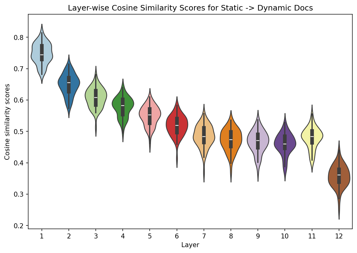
This plot shows how, at every subsequent layer in our model, poem embeddings further diverge from the original embeddings furnished by the model. One way to interpret this progression is via context: at every layer, the model further specifies context for the inputs, until the link between the context-less embeddings and the contextual ones becomes quite weak.
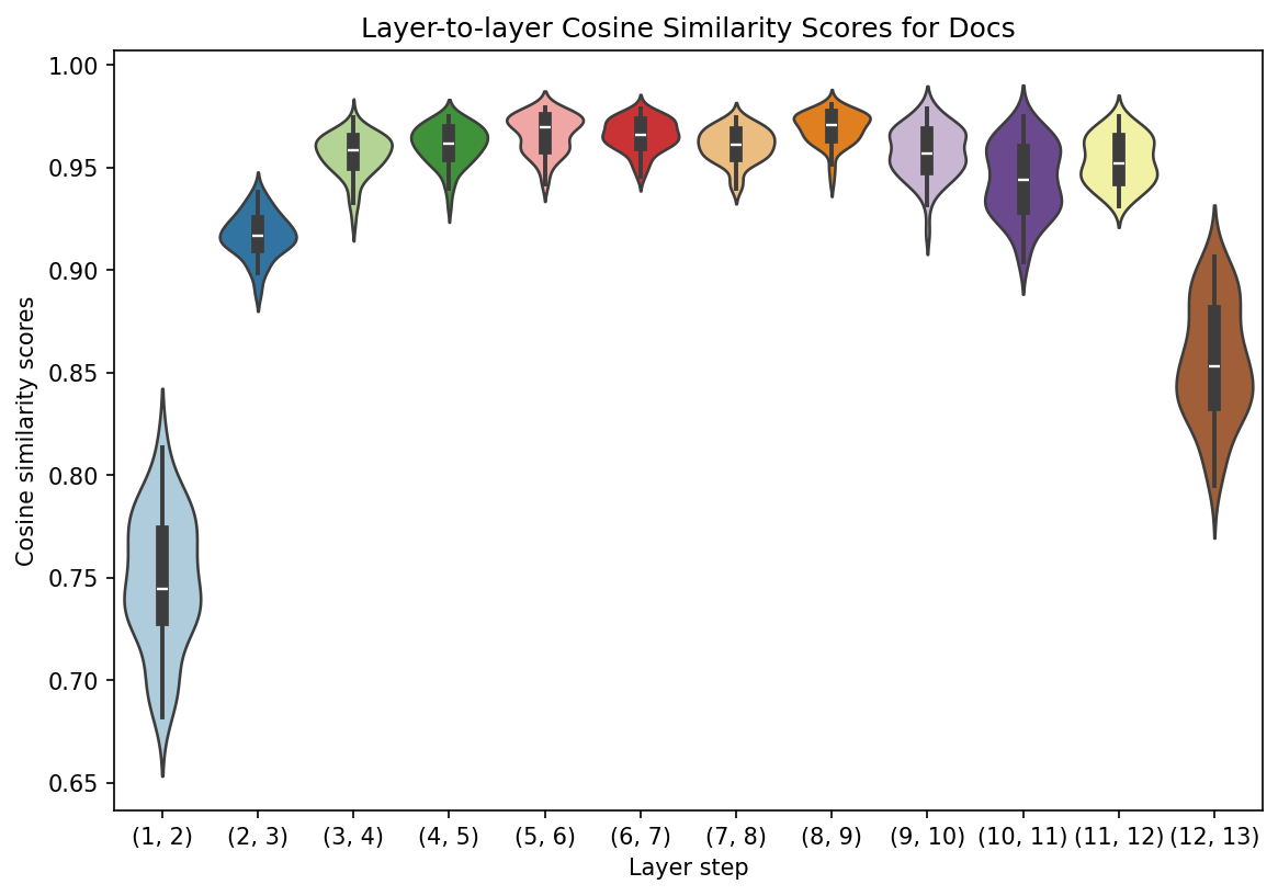
Slightly modifying the above procedure will show this layer-by-layer change. Below, we make our comparisons from one layer to the next.
layer2layer = []
previous = original_embeddings
for idx, layer in enumerate(outputs.hidden_states[1:]):
    # Pool the layer
    layer = mean_pool(layer, attention_mask)

    scores = []
    for static, dynamic in zip(previous, layer):
        # Compute cosine similarity
        similarities = cosine_similarity([static, dynamic])

        # `similarities` is a (2, 2) square matrix. We get the lower left
        # value, set up a step tracker, and append both
        score = similarities[np.tril_indices(2, k = -1)].item()
        step = f"({idx + 1}, {idx + 2})"
        scores.append((step, score))

    # Add the layer transition scores to our running list
    layer2layer.extend(scores)

    # Set the current layer to `previous`
    previous = layer
Reformat.
layer2layer = pd.DataFrame(
    layer2layer, columns = ["step", "cosine_similarity"]
)
And plot.
plt.figure(figsize = (9, 6))
g = sns.violinplot(
    data = layer2layer,
    x = "step",
    y = "cosine_similarity",
    hue = "step",
    palette = "Paired",
    legend = False
)
g.set(
    title = "Layer-to-layer Cosine Similarity Scores for Docs",
    xlabel = "Layer step",
    ylabel = "Cosine similarity scores"
)
plt.show()