4. N-gram Models

This chapter discusses n-gram models. We will create unigram (single-token) and bigram (two-token) sequences from a corpus, about which we compute measures like probability, information, entropy, and perplexity. Using these measures as weighting for different sampling strategies, we implement a few simple text generators.

• Data: 59 Emily Dickinson poems collected from the Poetry Foundation

• Credits: Portions of this chapter are adapted from Rafael Alvarado’s Exploratory Text Analytics

4.1. Preliminaries

Here are the libraries we need:

from pathlib import Path

import nltk
import numpy as np
import pandas as pd
import seaborn as sns
import matplotlib.pyplot as plt

Two helper functions will load the corpus and prepare it for modeling. They should be familiar: we defined them in the last chapter.

Show helper functions

def load_corpus(paths):
    """Load a corpus from paths.

    Parameters
    ----------
    paths : list[Path]
        A list of paths

    Returns
    -------
    corpus : list[str]
        The corpus
    """
    # Initialize an empty list to store the corpus
    corpus = []
    
    # March through each path, open the file, and load it
    for path in paths:
        with path.open("r") as fin:
            doc = fin.read()
            # Then add the file to the list
            corpus.append(doc)

    # Return the result: a list of strings, where each string is the contents
    # of a file
    return corpus


def preprocess(doc, ngram = 1):
    """Preprocess a document.

    Parameters
    ----------
    doc : str
        The document to preprocess
    ngram : int
        How many n-grams to break the document into
    
    Returns
    -------
    tokens : list
        Tokenized document
    """
    # First, change the case of the words to lowercase
    doc = doc.lower()

    # Tokenize the string. Optionally, make 2-gram (or more) sequences from
    # those tokens
    tokens = nltk.word_tokenize(doc)
    if ngram > 1:
        tokens = list(nltk.ngrams(tokens, ngram))
    
    return tokens

Now, set up the data directory and load a file manifest.

datadir = Path("data/texts/dickinson")
metadata = pd.read_csv(datadir / "metadata.csv")

metadata.info()

<class 'pandas.core.frame.DataFrame'>
RangeIndex: 59 entries, 0 to 58
Data columns (total 3 columns):
 #   Column  Non-Null Count  Dtype  
---  ------  --------------  -----  
 0   title   59 non-null     object 
 1   number  57 non-null     float64
 2   file    59 non-null     object 
dtypes: float64(1), object(2)
memory usage: 1.5+ KB

We won’t be using much of this data, but it helps keep our work aligned. Here’s a snippet:

metadata.head()

	title	number	file
0	After great pain, a formal feeling comes –	372.0	00.txt
1	All overgrown by cunning moss,	146.0	01.txt
2	Banish Air from Air	963.0	02.txt
3	Because I could not stop for Death –	479.0	03.txt
4	Before I got my eye put out –	336.0	04.txt

Now, load the corpus.

paths = [datadir / "poems" / fname for fname in metadata["file"]]
corpus = load_corpus(paths)

And we’re ready!

4.2. Unigrams

First: unigrams. Below, we preprocess the corpus into lists of tokens. Note that, unlike with the obituaries, we are keeping the punctuation.

unigrams = [preprocess(poem, ngram = 1) for poem in corpus]

Example:

idx = np.random.choice(len(corpus))
print(unigrams[idx])

['i', 'counted', 'till', 'they', 'danced', 'so', 'their', 'slippers', 'leaped', 'the', 'town', '–', 'and', 'then', 'i', 'took', 'a', 'pencil', 'to', 'note', 'the', 'rebels', 'down', '–', 'and', 'then', 'they', 'grew', 'so', 'jolly', 'i', 'did', 'resign', 'the', 'prig', '–', 'and', 'ten', 'of', 'my', 'once', 'stately', 'toes', 'are', 'marshalled', 'for', 'a', 'jig', '!']

4.2.1. Unigram metrics

We convert to a DataFrame to run computations on these tokens. The cell below performs the following operations:

1. Make a DataFrame by assigning the token lists to a column, w1

2. Use .explode() to unpack those lists into individual rows

3. Count the number of times each token appears with .value_counts()

4. Use .to_frame() to convert the counts (which is a Series) back to a DataFrame, storing the counts in a new column, n

unigram_df = pd.DataFrame({"w1": unigrams})
unigram_df = (
    unigram_df
    .explode("w1")
    .value_counts("w1")
    .to_frame("n")
)

Fully formatted:

unigram_df.head()

	n
w1
-	269
the	265
–	235
,	189
and	137

With the data formatted, we can compute metrics about these tokens.

Computing the probability of tokens is simple. For token \(w\), we find its count \(n\) and divide that by the total number of tokens in the corpus, \(C\).

\[ P(w) = \frac{n(w)}{C} \]

Implementing in code is straightforward:

C = unigram_df["n"].sum()
unigram_df["prob"] = unigram_df["n"] / C

A token’s surprise is its inverse probability.

\[ S(w) = \frac{1}{P(w)} \]

We use this to calculate information, which is the log-normalized surprise of a token. Note our use of \(\log_2\). This is to express information in terms of bits.

\[ I(w) = \log_2(S(w)) \]

Doing this in code is also straightforward:

unigram_df["info"] = np.log2(1 / unigram_df["prob"])

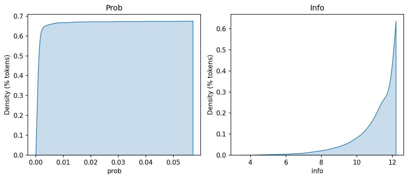
If we look at the information values, we will see that most are quite high. This should make sense. Information is just the normalized surprise of a token, which increases as its probability decreases. Because most tokens have low probability, they have high information.

fig, axes = plt.subplots(1, 2, figsize = (9, 4))
token_idx = range(len(unigram_df))

for idx, measure in zip([0, 1], ["prob", "info"]):
    sns.kdeplot(
        unigram_df[measure],
        fill = True,
        cumulative = True,
        clip = (0, np.max(unigram_df[measure])),
        ax = axes[idx]
    )
    axes[idx].set(
        title = measure.capitalize(),
        ylabel = "Density (% tokens)"
    )

plt.tight_layout()
plt.show()

Self-entropy \(h\) is a token’s information value, calculated by multiplying its probability by its information:

\[ h(w) = P(w) \cdot I(w) \]

The sum of all self-entropy values is the entropy \(H\), an overall measure of uncertainty in our token frequencies. It is the weighted average of the number of bits required to encode some data.

\[ H = \sum_{w} P(w) \cdot I(w) \]

Why not take the average of \(I\)? Look at the skew in tokens frequency. Certain tokens make disproportionate contributions to the overall distribution of values in our data, which a raw average would not reflect.

In code, calculating entropy looks like the following:

unigram_df["self-entropy"] = unigram_df["prob"] * unigram_df["info"]
print("Entropy of unigrams:", unigram_df["self-entropy"].sum())

Entropy of unigrams: 8.392710150066268

4.2.2. Generation

Having the probability distribution of unigrams in our corpus enables to do text generation—of a very primitive kind. Technically, generation here just means sampling from the distribution. We weight our sampling function with token probabilities so that more probable tokens are sampled more frequently than less probable ones. If we didn’t do that weighting, the sampling function would simply choose tokens at random.

Our sampling function is the .sample() method in pandas. Below, we sample 10 tokens and use the values in prob as our weighting. We set replace to True to allow a token to be sampled multiple times.

sampled = unigram_df.sample(n = 10, weights = "prob", replace = True)
seq = sampled.index
print(" ".join(seq))

in a us those done to price would . had

But, really, is the above any better than an unweighted sampling?

sampled = unigram_df.sample(n = 10, weights = None, replace = True)
seq = sampled.index
print(" ".join(seq))

tilling pontoon built forever grass command ” traveller debate remove

…maybe? It’s hard to tell by reading the outputs alone. But what we can do is use another metric, cross-entropy, to measure how well these two sampling strategies do against a baseline probability distribution. Cross-entropy is closely related to entropy. It measures the average amount of information needed to encode one probability distribution into another. That is, it is a measure of how well one distribution approximates the other.

We express cross-entropy as follows:

\[ H_{\text{cross}}(P, Q) = -\sum_w P(w)\log_2(Q(w)) \]

Where:

• \(H_{\text{cross}}(P, Q)\) is the cross-entropy between the true distribution \(P\) and the estimated distribution \(Q\)

• \(P(w)\) is the true probability of the token \(w\)

• \(Q(w)\) is the estimated probability of the token \(w\)

In this small experiment, “predicted” probabilities will just be the average probability of a token in the corpus. This acts as a baseline against which we can measure the sampling strategies.

4.2.3. Unigram modeling

Let’s set up the pieces we need. First, we define how many tokens N will be sampled for each strategy. Then we create a vector of the mean token probabilities in our corpus and repeat that value N times.

N = 10
baseline = np.repeat(unigram_df["prob"].mean(), N)
print(baseline)

[0.00067843 0.00067843 0.00067843 0.00067843 0.00067843 0.00067843
 0.00067843 0.00067843 0.00067843 0.00067843]

Now we define a function to calculate cross-entropy:

def calculate_cross_entropy(Pw, Qw):
    """Calculate the cross-entropy of distribution against another.

    Parameters
    ----------
    Pw : np.ndarray
        True values of the distribution
    Qw : np.ndarray
        Predicted distribution

    Returns
    -------
    cross_entropy : float
        The cross-entropy
    """
    log_Qw = np.log2(Qw)
    Sigma = np.sum(Pw * log_Qw)
    cross_entropy = -Sigma
    
    return cross_entropy

Here is some example output:

cross_entropy = calculate_cross_entropy(baseline, sampled["prob"])
print("Cross-entropy:", cross_entropy)

Cross-entropy: 0.07967390580694189

But to do our test, we will calculate the cross-entropy scores for our two sampling functions many times in a for loop:

samplers = {"weighted": "prob", "unweighted": None}
results = {"weighted": [], "unweighted": []}

for strategy, sampler in samplers.items():
    for _ in range(100):
        sequence = unigram_df.sample(n = N, weights = sampler, replace = True)
        cross_entropy = calculate_cross_entropy(baseline, sequence["prob"])
        results[strategy].append(cross_entropy)

Cross-entropy is a common loss function in language modeling, but when it’s used to report on model performance you will most often see it transformed into perplexity. Perplexity is cross-entropy’s exponentiation:

\[ PP = 2^{H_{\text{cross}}} \]

The value this produces is the average number of choices a model has to make to predict the next token in a generated sequence. Below, we calculate perplexity over the average cross-entropy scores form the sampling run above.

perplexity = pd.DataFrame(results)
for col in perplexity.columns:
    perplexity[col] = np.exp2(perplexity[col].mean())

print(perplexity.mean().sort_values())

weighted      1.041005
unweighted    1.056168
dtype: float64

When compared against the average probability of tokens in our corpus, our weighted sampling strategy has slightly less perplexity than our unweighted one. That tells us it is somewhat easier to represent our baseline distribution with the weighted samples than with the unweighted ones. In other words, the weighted samples are a better approximation of the mean probability of tokens in our corpus.

Cross-entropy and perplexity are two ways to validate such a model, but they are not necessarily the final determinants for what makes a good model. Neither sampling strategy gives us readable outputs, for example, and this is because the underlying data does not capture sequential relationships between tokens, which we readers expect. Any sampling strategy can only improve a unigram distribution by so much if those relationships are absent in the data.

4.3. Bigrams

We now turn to bigrams, or sequences of two tokens. Representing the corpus as bigrams will produce a model that encodes sequential information about Dickinson’s poetry.

As before, we preprocess the corpus, but this time we set ngram = 2.

bigrams = [preprocess(poem, ngram = 2) for poem in corpus]

An example:

idx = np.random.choice(len(corpus))
print(bigrams[idx])

[('success', 'is'), ('is', 'counted'), ('counted', 'sweetest'), ('sweetest', 'by'), ('by', 'those'), ('those', 'who'), ('who', "ne'er"), ("ne'er", 'succeed'), ('succeed', '.'), ('.', 'to'), ('to', 'comprehend'), ('comprehend', 'a'), ('a', 'nectar'), ('nectar', 'requires'), ('requires', 'sorest'), ('sorest', 'need'), ('need', '.'), ('.', 'not'), ('not', 'one'), ('one', 'of'), ('of', 'all'), ('all', 'the'), ('the', 'purple'), ('purple', 'host'), ('host', 'who'), ('who', 'took'), ('took', 'the'), ('the', 'flag'), ('flag', 'today'), ('today', 'can'), ('can', 'tell'), ('tell', 'the'), ('the', 'definition'), ('definition', 'so'), ('so', 'clear'), ('clear', 'of'), ('of', 'victory'), ('victory', 'as'), ('as', 'he'), ('he', 'defeated'), ('defeated', '–'), ('–', 'dying'), ('dying', '–'), ('–', 'on'), ('on', 'whose'), ('whose', 'forbidden'), ('forbidden', 'ear'), ('ear', 'the'), ('the', 'distant'), ('distant', 'strains'), ('strains', 'of'), ('of', 'triumph'), ('triumph', 'burst'), ('burst', 'agonized'), ('agonized', 'and'), ('and', 'clear'), ('clear', '!')]

4.3.1. Bigram metrics

Counting bigrams involves more footwork. Below, we do the following:

1. Make a DataFrame by assigning the bigram lists to a column, bigram

2. Use .explode() to unpack those lists into individual rows

3. Split each bigram into a w1 and w2 column by casting them to a Series with .apply()

4. Use .groupby() on those two columns and take the .size() to count them

5. Convert the counts back to a DataFrame with .to_frame() with a new count column, n

bigram_df = pd.DataFrame({"bigram": bigrams}).explode("bigram")
bigram_df[["w1", "w2"]] = bigram_df["bigram"].apply(pd.Series)
bigram_df = (
    bigram_df
    .groupby(["w1", "w2"])
    .size()
    .to_frame("n")
)

Fully formatted:

bigram_df.head()

		n
w1	w2
!	but	2
	could	1
	futile	1
	i	1
	lips	1

From here, we could calculate the metrics on our bigrams in the same way that we did for our unigrams. But that wouldn’t establish a relationship from the first token in the bigram to the second token, it would just produce data about the frequency of bigrams in the corpus.

To establish that relationship, we must calculate the conditional probability of the two tokens in a bigram. That is, given token w1, how likely is token w2 to follow?

\[ p(w2|w1) = \frac{P(w1, w2)}{P(w1)} \]

This is easy to do with pandas: divide bigram frequencies by token frequencies in the unigram DataFrame.

bigram_df["prob"] = bigram_df["n"] / unigram_df["n"]

With conditional probabilities made, we can again get the information values. But this time, those values will describe the relationship between the first and second words in a bigram with respect to all such relationships in the corpus.

bigram_df["info"] = np.log2(1 / bigram_df["prob"])

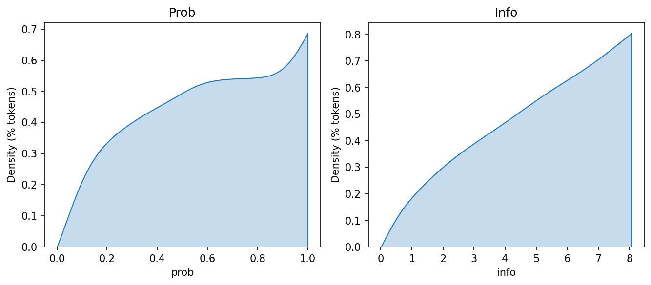
Plotting bigram probability and information produces a very different picture of the relationship between these two measures than the one we observed with unigrams.

fig, axes = plt.subplots(1, 2, figsize = (9, 4))
token_idx = range(len(bigram_df))

for idx, measure in zip([0, 1], ["prob", "info"]):
    sns.kdeplot(
        bigram_df[measure],
        fill = True,
        cumulative = True,
        clip = (0, np.max(bigram_df[measure])),
        ax = axes[idx]
    )
    axes[idx].set(
        title = measure.capitalize(),
        ylabel = "Density (% tokens)"
    )

plt.tight_layout()
plt.show()

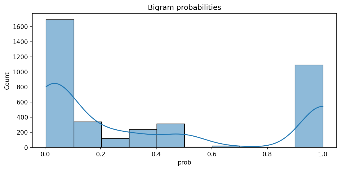
Why is this? Well, take a look at a histogram of the bigram probabilities. It’s (roughly) a bimodal distribution, with many bigrams clustering around the minimum and maximum probability values.

plt.figure(figsize = (9, 4))
g = sns.histplot(bigram_df["prob"], bins = 10, kde = True)
g.set(title = "Bigram probabilities")
plt.show()

Bigrams with \(p(w2|w1) \approx 1.0\) contain very little information. The second word always follows the first, so less information is required to encode this relationship. Likewise, bigrams with \(p(w2|w1) \approx 0.0\) have a lot of information: the second word follows many words, not just the first one, so more information is required to encode the possibility of observing this particular sequence.

You may see where this is going: the bimodal distribution means there is a broad range of information values, with values clustered at the two ends of the data. This creates a gradually increasing line in the cumulative density plot above. As we move to bigram generation, keep this in mind.

4.3.2. Generation

Another way to think about the information weighting between bigrams is to consider bigrams as a directed graph, in which a w1 token branches into various w2 tokens. The graph below shows a few successors from the token “the” and the successors of those successors. Arrows indicate the direction of a sequence. Edge thickness corresponds to the information of the relationship between the two tokens in a bigram.

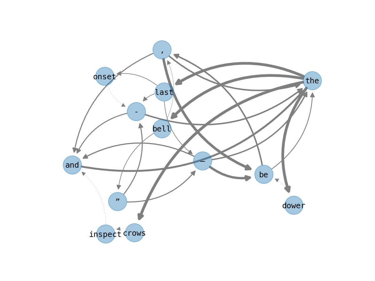
Note the variation in thickness, which is also a proxy for the probability that w2 follows from w1. Below is an improbable bigram. It requires a lot of information to encode:

bigram_df.loc[(slice(None), "dower"), :]

		n	prob	info
w1	w2
the	dower	1	0.003774	8.049849

Now: an extremely probable one. It requires very little information (none at all, in fact):

bigram_df.loc[("crows", slice(None)), :]

		n	prob	info
w1	w2
crows	inspect	1	1.0	0.0

These two examples sit, respectively, at the maximum and minimum limit of the histogram above. Other bigrams in this graph are somewhere in between.

Bigram generation involves traversing this graph. The general procedure is this: given a token, we use the conditional probabilities of all other tokens in the corpus as weights for our sampling function. Many weights will be zero, meaning it isn’t possible to move from one particular token to another. But for those weights that aren’t zero, we make a selection. Then, we use that new token as the basis for another selection, and so on. This is, in effect, a rudimentary Markov chain.

Doing this is easier with a wide format for the bigram DataFrame. In this format, rows are w1 in the bigrams and the columns are w2. Each cell in this new DataFrame will represent the conditional probability of moving from w1 to w2. The resultant DataFrame will be quite large.

bigram_probs = bigram_df["prob"].unstack(fill_value = 0)

print("Shape:", bigram_probs.shape)

Shape: (1473, 1466)

Time to implement the generation function.

def generate(unigram_df, bigram_df, bigram_probs, N = 10):
    """Generate `N` new tokens.

    Parameters
    ----------
    unigram_df : pd.DataFrame
        The unigram data
    bigram_df : pd.DataFrame
        The bigram data
    bigram_probs : pd.DataFrame
        Conditional probabilities of the bigrams
    N : int
        Number of tokens to generate

    Returns
    -------
    generated : tuple
        Generated tokens and some corresponding data
    """
    # Randomly select a token row from the unigram DataFrame, using token
    # frequency as a weighting. This means more frequent tokens are more likely
    # to be sampled than infrequent ones
    seed = unigram_df.sample(weights = "n")
    seed = seed.index.item()

    # Initialize two empty lists to store our results. One will be the
    # generated sequence, the other will be some metadata about that sequence
    sequence = []
    metadata = []

    # Iterate N times.
    while N > 0:
        # First, does our seed appear as the leading token in a bigram? If not,
        # we have to try a new seed
        if seed not in bigram_probs.index:
            seed = unigram_df[unigram_df.index != seed].sample(weights = "n")
            seed = seed.index.item()

        # Add the seed to the sequence
        sequence.append(seed)

        # Get the row in the bigram probabilities that corresponds to our
        # token, then sample from this token using the probabilities as
        # weights
        next_token_row = bigram_probs.loc[seed]
        next_token = next_token_row.sample(weights = next_token_row.values)
        next_token = next_token.index.item()

        # Get the probability and information of the resultant bigram
        bigram_prob = bigram_df.loc[(seed, next_token), "prob"]
        bigram_info = bigram_df.loc[(seed, next_token), "info"]

        # Store the above information in the metadata list, along with the
        # bigram
        metadata.append({
            "bigram": (seed, next_token),
            "prob": bigram_prob,
            "info": bigram_info
        })

        # Set the next token to the new seed and decrease our counter
        seed = next_token
        N -= 1

    # Convert the metadata to a DataFrame and return it with the sequence
    metadata = pd.DataFrame(metadata)

    return sequence, metadata

Let’s run this code a few times and look at the sequences first.

for _ in range(5):
    sequence, _ = generate(unigram_df, bigram_df, bigram_probs)
    print(" ".join(sequence))

note the chillest land - in the day i ,
i thought so clear of industries enacted opon a mouse
expectation – oh , all the miles - who took
of sight of prisons broad by those old — and
after death – exhale in the suns — i dwell

Not bad! This reads considerably better than the unigram output. But can we do better? Let’s explore a few different bigram sampling strategies to find out.

4.4. Sampling Strategies

We will look at three different strategies for sampling:

1. Weighted sampling

2. Greedy sampling

3. Top-k sampling

4.4.1. Weighted sampling

The first should be familiar. It’s what we have been using all along. In weighted sampling, every token/bigram is assigned a weighted value, which corresponds to its probability in the corpus. Higher probabilities mean that the token/bigram is sampled more frequently than ones with lower probabilities.

def sample_weighted(weights, idx):
    """Perform weighted sampling.

    Parameters
    ----------
    weights : pd.DataFrame
        DataFrame of weights
    idx : int or str
        An index to a row in `data`

    Returns
    -------
    token
        The sampled token
    """
    row = weights.loc[idx]
    token = row.sample(n = 1, weights = row.values)
    token = token.index.item()

    return token

It looks like so:

sample = sample_weighted(bigram_probs, "air")
print(sample)

–

4.4.2. Greedy sampling

Greedy sampling always selects the most probable token. In a sense, it isn’t really sampling at all.

def sample_greedy(weights, idx):
    """Perform greedy sampling.

    Parameters
    ----------
    weights : pd.DataFrame
        DataFrame of weights
    idx : int or str
        An index to a row in `data`

    Returns
    -------
    token
        The sampled token
    """
    row = weights.loc[idx]
    max_value = np.argmax(row)
    token = row.index[max_value]

    return token

An example:

for _ in range(5):
    sample = sample_greedy(bigram_probs, "air")
    print(sample)

-
-
-
-
-

4.4.3. Top-k sampling

Finally, top-k sampling works much like weighted sampling, except it first performs a cutoff to the k highest values in the candidate pool.

def sample_topk(weights, idx, k = 10):
    """Perform top-k sampling.

    Parameters
    ----------
    weights : pd.DataFrame
        DataFrame of weights
    idx : int or str
        An index to a row in `data`
    k : int
        The number of highest-values candidates from which to sample

    Returns
    -------
    token
        The sampled token
    """
    row = weights.loc[idx]
    topk = row.nlargest(k)
    token = topk.sample(n = 1, weights = topk.values)
    token = token.index.item()

    return token

Here are a few examples:

for _ in range(5):
    sample = sample_topk(bigram_probs, "air")
    print(sample)

from
–
–
with
,

4.4.4. Generation with different sampling strategies

Let’s now look at the results of these sampling strategies. To do so, we will rewrite the generate() function above to accept a new argument, sampler, which will correspond to one of the above sampling strategies.

def generate_from_sampler(
    unigram_df, bigram_df, bigram_probs, sampler, N = 10
):
    """Generate `N` new tokens.

    Parameters
    ----------
    unigram_df : pd.DataFrame
        The unigram data
    bigram_df : pd.DataFrame
        The bigram data
    bigram_probs : pd.DataFrame
        Conditional probabilities of the bigrams
    sampler : Callable
        A sampling function
    N : int
        Number of tokens to generate

    Returns
    -------
    generated : tuple
        Generated tokens and some corresponding data
    """
    # Randomly select a token row from the unigram DataFrame, using token
    # frequency as a weighting. This means more frequent tokens are more likely
    # to be sampled than infrequent ones
    seed = unigram_df.sample(weights = "n")
    seed = seed.index.item()

    # Initialize two empty lists to store our results. One will be the
    # generated sequence, the other will be some metadata about that sequence
    sequence = []
    metadata = []

    # Iterate N times.
    while N > 0:
        # First, does our seed appear as the leading token in a bigram? If not,
        # we have to try a new seed
        if seed not in bigram_probs.index:
            seed = unigram_df[unigram_df.index != seed].sample(weights = "n")
            seed = seed.index.item()

        # Add the seed to the sequence
        sequence.append(seed)

        # Get the row in the bigram probabilities that corresponds to our
        # token, then sample from this token using the sampler
        next_token = sampler(bigram_probs, seed)

        # Get the probability and information of the resultant bigram
        bigram_prob = bigram_df.loc[(seed, next_token), "prob"]
        bigram_info = bigram_df.loc[(seed, next_token), "info"]

        # Store the above information in the metadata list, along with the
        # bigram
        metadata.append({
            "bigram": (seed, next_token),
            "prob": bigram_prob,
            "info": bigram_info
        })

        # Set the next token to the new seed and decrease our counter
        seed = next_token
        N -= 1

    # Convert the metadata to a DataFrame and return it with the sequence
    metadata = pd.DataFrame(metadata)

    return sequence, metadata

A for loop that runs this function over our different samplers is below:

samplers = {
    "weighted": sample_weighted,
    "greedy": sample_greedy,
    "topk": sample_topk
}
for strategy, sampler in samplers.items():
    print("Strategy:", strategy)
    for _ in range(5):
        sequence, metadata =  generate_from_sampler(
            unigram_df, bigram_df, bigram_probs, sampler, N = 15
        )
        print("+", " ".join(sequence))
    print("\n")

Strategy: weighted
+ years would strike us of visitors – between eternity – 't is a summer ’
+ a gayer scarf - stopless - or be , leap , and slowness – then
+ of my eye – of me , it , mechanical , a truffled hut it
+ not know no other latitudes – since then i than they take the pulpit -
+ in circuit lies too – or rather be justifying for breakfast , like boanerges -


Strategy: greedy
+ fall - and then the soul - and then the soul - and then the
+ corn - and then the soul - and then the soul - and then the
+ me – and then the soul - and then the soul - and then the
+ sip , and then the soul - and then the soul - and then the
+ as a bird , and then the soul - and then the soul - and


Strategy: topk
+ could she one in my brain , and i have lodged a house – then
+ here – then the sun – he defeated – and then i , a crumb
+ royal seal ! might as all the air from the soul 's law — it
+ s cheek is the stillness is the one raised softly to be , and every

+ - and he dare in the soul opon the house that have borne - i

Remember the earlier point about bigrams with \(p(w2|w1) \approx 1.0\)? That clearly influences the greedy sampling output. The generator gets trapped in a loop of bigrams that have exceedingly high probabilities.

4.4.5. Measuring sampling strategies

Finally, we look at the cross-entropy of these various sampling strategies. As before, we use a baseline that corresponds to the mean bigram probabilities in the corpus.

N = 10
baseline = np.repeat(bigram_df["prob"].mean(), N)
print(baseline)

[0.38676428 0.38676428 0.38676428 0.38676428 0.38676428 0.38676428
 0.38676428 0.38676428 0.38676428 0.38676428]

A for loop will implement the generation:

results = {"weighted": [], "greedy": [], "topk": []}
for strategy, sampler in samplers.items():
    for _ in range(100):
        sequence, metadata = generate_from_sampler(
            unigram_df, bigram_df, bigram_probs, sampler, N = N
        )
        cross_entropy = calculate_cross_entropy(baseline, metadata["prob"])
        results[strategy].append(cross_entropy)

Now we look at the results, which we transform into perplexity scores.

perplexity = pd.DataFrame(results)
for col in perplexity.columns:
    perplexity[col] = np.exp2(perplexity[col].mean())

print(perplexity.mean().sort_values())

greedy      4115.834739
weighted    5047.784690
topk        5189.935375
dtype: float64

These are poor—but unsurprising—results. With the bigram probabilities skewing to one-to-one relationships or one-to-dozens, there is effectively no way to generalize across all types of bigrams in the corpus.

But consider what the results do tell us: greedy sampling performs the best by this metric. Since it always picks the most likely token, its selection will push toward the center of the probability mass, whereas the other two strategies allow tokens from outside that center. Even so, the latter two strategies produce more readable text, at least by our standards as human readers. This ends up being an important lesson: a model that performs well with respect to metrics does not necessarily mean it is a good model.