11. Attention in Vector Space#
This chapter demonstrates attention in terms of vector space operations.
11.1. Preliminaries#
We need the following libraries.
import torch
import torch.nn.functional as F
import numpy as np
import pandas as pd
from transformers import AutoTokenizer, AutoModel
from sklearn.decomposition import PCA
import matplotlib.pyplot as plt
import seaborn as sns
We’ll use BERT for our demonstration.
checkpoint = "bert-base-uncased"
tokenizer = AutoTokenizer.from_pretrained(checkpoint)
model = AutoModel.from_pretrained(checkpoint, attn_implementation = "eager")
11.2. Extracting Attention#
With the model loaded, we process a sentence.
sentence = "Oh, this book? I've enjoyed it."
inputs = tokenizer(sentence, return_tensors = "pt")
with torch.no_grad():
    outputs = model(**inputs, output_attentions = True)
Now, we extract the layer attentions and build a list of tokens.
attentions = [attn.squeeze(0).numpy() for attn in outputs.attentions]
labels = [tokenizer.decode(tokid) for tokid in inputs["input_ids"].squeeze(0)]
We’ll drop the [CLS] and [SEP] tokens for this demonstration.
attentions = [attn[:, 1:-1, 1:-1] for attn in attentions]
labels = labels[1:-1]
11.3. Plotting Functions#
We need to define two functions for visualizing attention in vector space. The first one transforms attention embeddings into two-dimensional vectors.
def to_xy_coords(scores, summary_stat = np.mean, norm = True):
    """Reduce the dimensionality of attention scores for plotting.

    Parameters
    ----------
    scores : np.ndarray
        Multihead scores for a layer
    summary_stat : Callable
        What statistic to use to summarize the multiple attention heads
    norm : bool
        Whether to normalize the scores
    """
    # Calculate our summary stat. We need to do this to handle scores across
    # the multiple attention heads
    scores = summary_stat(scores, axis = 0)

    # Reduce the dimensions of the data to XY coordinates
    pca = PCA(n_components = 2)
    xy = pca.fit_transform(scores)

    # Are we normalizing?
    if norm:
        norm_by = np.linalg.norm(xy)
        xy /= norm_by

    return xy
The second is the plotting function itself.
def plot_vectors(
    *vectors,
    labels = [],
    colors = [],
    figsize = (3, 3),
    fig = None,
    ax = None,
    title = None,
):
    """Plot 2-dimensional vectors.

    Parameters
    ----------
    vectors : nd.ndarray
        Vectors to plot
    labels : list
        Labels for the vectors
    colors : list
        Vector colors (string names like "black", "red", etc.)
    fig : matplotlib.figure.Figure, optional
        Existing figure object to use for the plot
    ax : matplotlib.axes.Axes, optional
        Existing axis object to use for the plot
    title : str, optional
        Subplot title

    Returns
    -------
    fig, ax : tuple
        The figure and axis
    """
    # Wrap vectors into a single array
    vectors = np.array(vectors)
    n_vector, n_dim = vectors.shape
    if n_dim != 2:
        raise ValueError("We can only plot 2-dimensional vectors")

    # Create a new figure and axis if not provided
    if fig is None or ax is None:
        fig, ax = plt.subplots(figsize = figsize)

    # Populate colors
    if not colors:
        colors = ["black"] * n_vector

    # Create a (0, 0) origin point for each vector
    origin = np.zeros((2, n_vector))

    # Then plot each vector, storing the handles and labels for each
    handles, handle_labels = [], []
    for idx, vector in enumerate(vectors):
        color = colors[idx]
        label = labels[idx] if labels else None
        arrow = ax.quiver(
            *origin[:, idx],
            vector[0],
            vector[1],
            color = color,
            scale = 1,
            units = "xy",
            label = label
        )
        handles.append(arrow)
        handle_labels.append(label)

    # Set plot limits
    limit = np.max(np.abs(vectors))
    ax.set_xlim([-limit, limit])
    ax.set_ylim([-limit, limit])

    # Set axes to be in the center of the plot
    ax.axhline(y = 0, color = "k", linewidth = 0.8)
    ax.axvline(x = 0, color = "k", linewidth = 0.8)

    # Remove the outer box
    for spine in ax.spines.values():
        spine.set_visible(False)

    # Set the title
    if title:
        ax.set_title(title)

    # Return the figure, axis, handles, and labels
    return fig, ax, handles, handle_labels
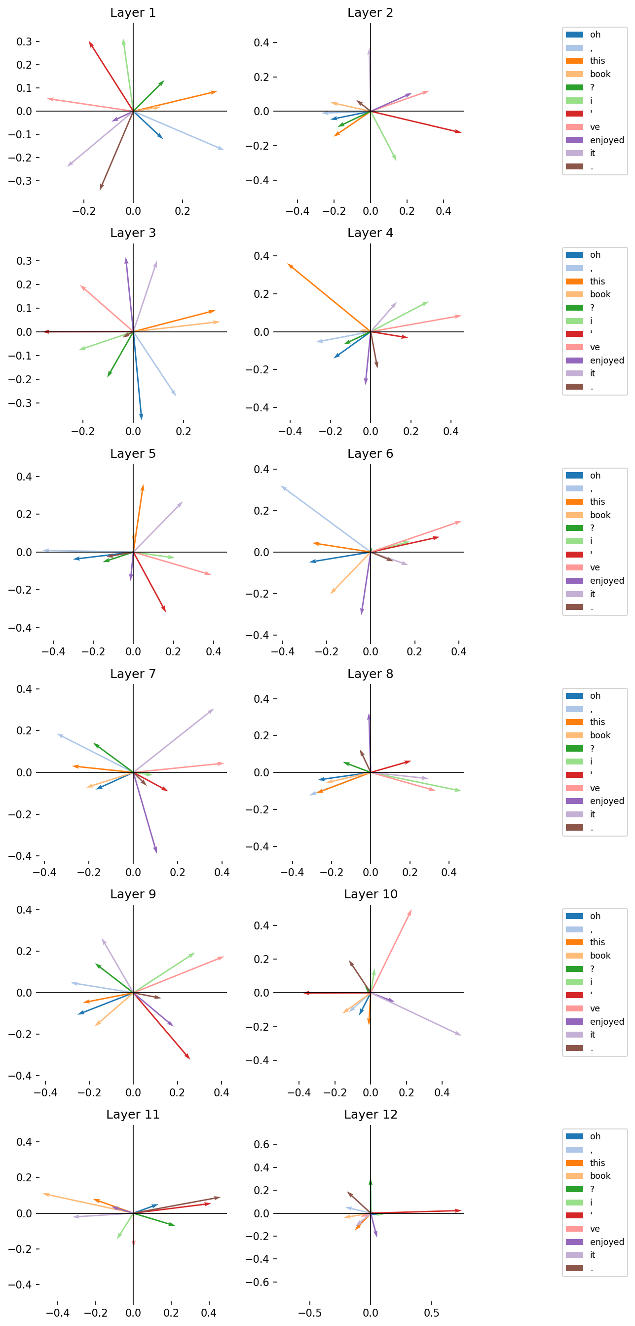
11.4. Visualizing Self-Attention#
With all of the above defined, we can now plot our attention scores in a two-dimensional vector space. Remember: in this space, proximity means similarity. During our vector space semantics session we derived this information using the dot product, which tells us how much of one vector is projected along another vector.
If you look back to the scaled_dot_product_attention() function in chapter 7,
you’ll see that calculating attention is a souped-up version of the dot
product. Those matrix multiplication calls are effectively dot product
operations, e.g. in the example below.
For a query matrix \(Q\):
A key matrix \(K\):
…and its transpose \(K^T\):
Multiplying the two together creates a scores matrix \(S\):
Or:
For pairs of query and key vectors, we get a dot product score. That means attention is just capturing information about how much the query vectors are projected along the key vectors. For a given token in the input, attention determines the orientation of that token to all other tokens. Then, it applies that information to the value matrix as a weighting.
# Set up a plot and roll through the attention layers
fig, axes = plt.subplots(6, 2, figsize = (9, 18))
for idx, (ax, layer) in enumerate(zip(axes.flatten(), attentions)):
    # Convert the attention scores to XY coordinates and produce some colors
    # for highlighting
    xy = list(to_xy_coords(layer))
    colors = sns.color_palette("tab20", len(xy))

    # Create a subplot for this layer
    fig, ax, handles, handle_labels = plot_vectors(
        *xy,
        colors = colors,
        labels = labels,
        fig = fig,
        ax = ax,
        title = f"Layer {idx + 1}"
    )

    # Annotate every row with the token labels
    if (idx + 1) % 2 != 0:
        continue
    ax.legend(
        handles,
        handle_labels,
        loc = "upper left",
        bbox_to_anchor = (1.5, 1),
        fontsize = "small",
    )

# Show the plot
plt.tight_layout()
plt.show()
11.5. Vector Projection#
Using the dot product, we can take two vectors, A and B, and create a third
“projection” vector, which shows how much of A sits along the direction of
B. Attention is capturing this kind of information as it runs, but it’s
helpful to see the projection ourselves.
Let’s define a function to create this vector below.
def vector_projection(A, B):
    """Project vector A onto B.

    Formula:
        (A•B / ||B||^2) * B

    Parameters
    ----------
    A, B: np.ndarray
        The two vectors

    Returns
    -------
    projection : np.ndarray
        The projection of A onto B
    """
    ab_dot = A @ B
    b_magnitude_squared = np.linalg.norm(B) ** 2
    projection = (ab_dot / b_magnitude_squared) * B

    return projection
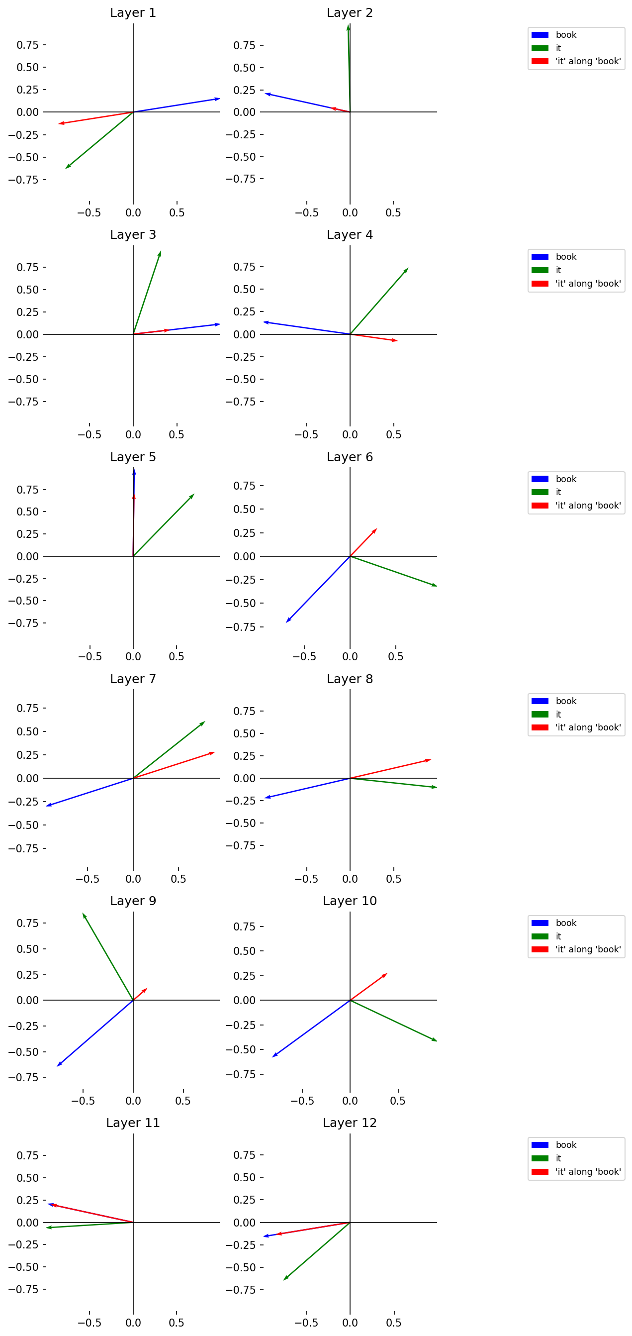
With the function defined, we project the attention vector for “it” onto the one for “book” across every layer in BERT. This will create a new projection vector whose orientation in vector space represents the amount of “it” along “book.” Keep the following in mind as you inspect the result:
If the projection vector tends toward the vector for “book,” this means more of “it” is captured along “book”
If the projection vector tends away from the vector for “book,” this means less of “it” is captured along “book”
Given the nature of attention, what we would expect is that, at certain layer, or set of layers, BERT will be able to determine that “book” and “it” refer to the same thing. A major goal in mechanistic interpretability is to find out the location of this behavior.
But for model training, the goal is this: the model should be better able to capture the relationship between two tokens. How? It furnishes vectors for each token, captures their relationship via the dot product to weight the vectors on the basis of that relationship (i.e., it calculates attention), and uses the weighted vectors to make a prediction. Then, based on how well it has made this prediction, the model makes adjustments to the initial vectors it uses to represent the tokens as well as the amount of weighting it uses to change those vectors when it calculates attention.
# Get the index positions for "book" and "it"
book_idx = 3
it_idx = 9

# Set up a plot and roll through the attention layers
fig, axes = plt.subplots(6, 2, figsize = (9, 18))
for idx, (ax, layer) in enumerate(zip(axes.flatten(), attentions)):
    # Convert the attention scores to XY coordinates. We turn off
    # normalization here because we're only focusing on two vectors, which
    # we'll normalize separately
    xy = list(to_xy_coords(layer, norm = False))

    # Select our two vectors, normalize them, and calculate the projection
    # vector
    book, it = xy[book_idx], xy[it_idx]
    book /= np.linalg.norm(book)
    it /= np.linalg.norm(it)
    projection = vector_projection(it, book)

    # Create our colors and labels
    colors = ["blue", "green", "red"]
    plot_labels = [labels[book_idx], labels[it_idx]]
    plot_labels += [f"'{labels[it_idx]}' along '{labels[book_idx]}'"]

    # Create a subplot for this layer
    fig, ax, handles, handle_labels = plot_vectors(
        book,
        it,
        projection,
        colors = colors,
        labels = plot_labels,
        fig = fig,
        ax = ax,
        title = f"Layer {idx + 1}"
    )

    # Annotate every row with the token labels
    if (idx + 1) % 2 != 0:
        continue
    ax.legend(
        handles,
        handle_labels,
        loc = "upper left",
        bbox_to_anchor = (1.5, 1),
        fontsize = "small",
    )

# Show the plot
plt.tight_layout()
plt.show()