6. Vector Space Semantics#
This chapter overviews vector space semantics. It introduces core operations on vectors and vector spaces and demonstrates how to use these operations to define a measure of of semantic similarity. We then turn to static word embeddings to discuss concept modeling as well as embedding analogies; a final experiment demonstrates how to disambiguate part-of-speech tags in embeddings.
Data: A document-term matrix representation of Melanie Walsh’s corpus of ~380 obituaries from the New York Times and tagged WordNet embeddings
Credits: Portions of this chapter are adapted from the UC Davis DataLab’s Natural Language Processing for Data Science
6.1. Preliminaries#
We need the following libraries:
import numpy as np
import pandas as pd
from sklearn.pipeline import make_pipeline
from sklearn.preprocessing import Normalizer
from sklearn.decomposition import PCA
from sklearn.metrics.pairwise import cosine_similarity
from sklearn.neighbors import NearestNeighbors
from sklearn.model_selection import train_test_split
from sklearn.linear_model import LogisticRegression
from sklearn.metrics import classification_report
from sklearn.feature_selection import RFE
from tabulate import tabulate
import matplotlib.pyplot as plt
import seaborn as sns
Our documents have already been vectorized into a document-term matrix (DTM). The only consideration is that the tokens have been lemmatized, that is, reduced to their uninflected forms.
dtm = pd.read_parquet("data/datasets/nyt_obituaries_dtm.parquet")
dtm.info()
<class 'pandas.core.frame.DataFrame'>
Index: 379 entries, Ada Lovelace to Karen Sparck Jones
Columns: 31165 entries, aachen to zwilich
dtypes: int64(31165)
memory usage: 90.1+ MB
6.2. Vector Space#
In the last chapter we plotted Henry James chapters in a two-dimensional scatter plot. We can do the same with our DTM using the function below.
def scatter_2d(matrix, norm = True, highlight = None, figsize = (5, 5)):
    """Plot a matrix in 2D vector space.

    Parameters
    ----------
    matrix : np.ndarray
        Matrix to plot
    norm : bool
        Whether to normalize the matrix values
    highlight : None or list
        List of indices to highlight
    figsize : tuple
        Figure size
    """
    # Find a way to reduce the matrix to two dimensions with PCA, adding
    # optional normalization along the way
    if norm:
        pipeline = make_pipeline(Normalizer(), PCA(n_components = 2))
    else:
        pipeline = make_pipeline(PCA(n_components = 2))
    reduced = pipeline.fit_transform(matrix)
    vis_data = pd.DataFrame(reduced, columns = ["x", "y"])

    # Plot
    plt.figure(figsize = figsize)
    g = sns.scatterplot(x = "x", y = "y", alpha = 0.8, data = vis_data)

    # Highlight markers, if applicable
    if highlight:
        selected = vis_data.iloc[highlight]
        sns.scatterplot(
            x = "x", y = "y", color = "red", data = selected
        )

    g.set(xlabel = "Dim. 1", ylabel = "Dim. 2")
    plt.show()
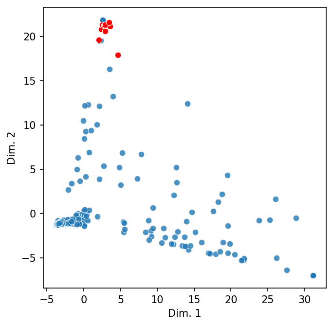
Below, we plot the DTM.
scatter_2d(dtm)

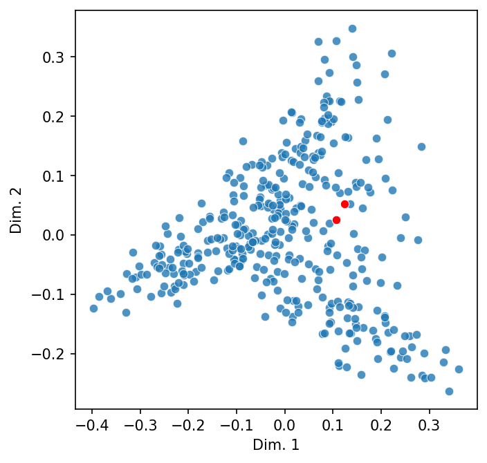
Doing so projects our matrix into a two-dimensional vector space. In the reigning metaphor of NLP, a space of this sort is a stand-in for meaning: the closer two points are in the scatter plot, the more similar they are in meaning.
Selecting the names of two related people in the obituaries will make this clear.
names = ["Bela Bartok", "Maurice Ravel"]
highlight = [dtm.index.get_loc(name) for name in names]
scatter_2d(dtm, highlight = highlight)
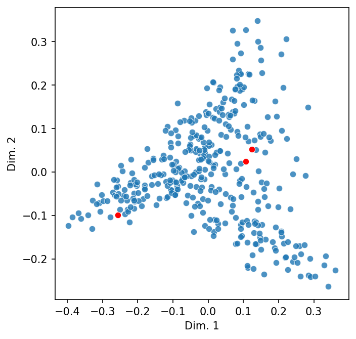
Let’s add in a third that we’d expect to be less similar.
names = ["Bela Bartok", "Maurice Ravel", "FDR"]
highlight = [dtm.index.get_loc(name) for name in names]
scatter_2d(dtm, highlight = highlight)
While we can only visualize these similarities in two- or three-dimensional spaces, which are called Euclidean spaces (i.e., they conform to physical space), the same idea—and importantly, the math—holds for similarity in high-dimensional spaces. But before we turn to what similarity means in vector space, we’ll overview how vectors work generally.
Our two example vectors will be the following:
A, B = dtm.loc["Lucille Ball"], dtm.loc["Carl Sagan"]
And we will limit ourselves to only two dimensions:
terms = ["television", "star"]
A, B = A[terms], B[terms]
6.2.1. Vector components#
A vector has a magnitude and a direction.
Magnitude
Description: The length of a vector from its origin to its end point. This is calculated as the square root of the sum of squares of its components
Notation: \(||A|| = \sqrt{a_1^2 + a_2^2 + \dots + a_n^2}\)
Result: Single value (scalar)
manual = np.sqrt(np.sum(np.square(A)))
numpy = np.linalg.norm(A)

assert manual == numpy, "Magnitudes don't match!"
print(numpy)
12.649110640673518
Direction
Description: The orientation of a vector in space. In Cartesian coordinates, it is the angles a vector forms across its axes. But direction can also be represented as a second unit vector, a vector of magnitude 1 that points in the same direction as the first. Most vector operations in NLP use the latter
Notation: \(\hat{A} = \frac{A}{||A||}\)
Result: Vector of length \(n\)
A / np.linalg.norm(A)
television    0.948683
star          0.316228
Name: Lucille Ball, dtype: float64
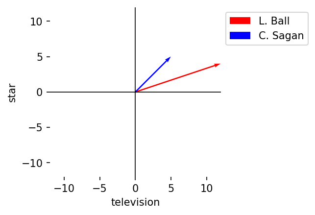
Let’s plot our two vectors to show their magnitude and orientation.
Show vector plot code
def plot_vectors(
    *vectors,
    vector_labels = [],
    axis_labels = [],
    colors = [],
    figsize = (3, 3)
):
    """Plot 2-dimensional vectors.

    Parameters
    ----------
    vectors : nd.ndarray
        Vectors to plot
    vector_labels : list
        Labels for the vectors
    axis_labels : list
        Labels for the axes in (x, y) order
    colors : list
        Vector colors (string names like "black", "red", etc.)
    figsize : tuple
        Figure size
    """
    # Wrap vectors into a single array
    vectors = np.array(vectors)
    n_vector, n_dim = vectors.shape
    if n_dim != 2:
        raise ValueError("We can only plot 2-dimensional vectors")

    # Populate colors
    if not colors:
        colors = ["black"] * n_vector

    # Create a (0, 0) origin point for each vector
    origin = np.zeros((2, n_vector))

    # Then plot each vector
    fig, ax = plt.subplots(figsize = figsize)
    for idx, vector in enumerate(vectors):
        color = colors[idx]
        ax.quiver(
            *origin[:, idx],
            vector[0],
            vector[1],
            color = color,
            scale = 1,
            units = "xy",
            label = vector_labels[idx] if vector_labels else None
        )

    # Set plot limits
    limit = np.max(np.abs(vectors))
    ax.set_xlim([-limit, limit])
    ax.set_ylim([-limit, limit])

    # Set axes to be in the center of the plot
    ax.axhline(y = 0, color = "k", linewidth = 0.8)
    ax.axvline(x = 0, color = "k", linewidth = 0.8)

    # Remove the outer box
    for spine in ax.spines.values():
        spine.set_visible(False)

    # Add axis labels, if applicable
    if axis_labels:
        xlab, ylab = axis_labels
        ax.set_xlabel(xlab)
        ax.set_ylabel(ylab)

    # Add a label legend, if applicable
    if vector_labels:
        ax.legend(loc = "upper left", bbox_to_anchor = (1, 1))

    # Show the plot
    plt.show()
vector_labels = ["L. Ball", "C. Sagan"]
colors = ["red", "blue"]
plot_vectors(
    A, B, vector_labels = vector_labels, axis_labels = terms, colors = colors
)
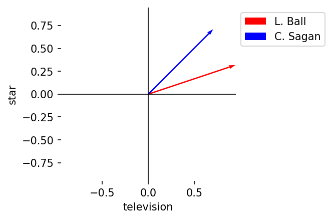
We can normalize our vectors by their direction. This will make the magnitude
of each vector equal to 1. You’ll see this operation called L2
normalization. (In scatter_2d above, this is what the Normalizer object
does.)
def l2_norm(vector):
    """Perform L2 normalization.

    Parameters
    ----------
    vector : np.ndarray
        Vector to normalize

    Returns
    -------
    vector : np.ndarray
        Normed vector
    """
    norm_by = np.linalg.norm(vector)
    return vector / norm_by
plot_vectors(
    l2_norm(A),
    l2_norm(B),
    vector_labels = vector_labels,
    axis_labels = terms,
    colors = colors
)
6.2.2. Vector operations#
We turn now to basic operations you can perform on/with vectors.
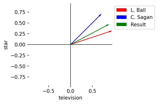
Summation
Description: Element-wise sums
Notation: \(A + B = (a_1 + b_1, a_2 + b_2, \dots, a_n + b_n)\)
Result: Vector of length \(n\)
C = A + B
plot_vectors(
    l2_norm(A),
    l2_norm(B),
    l2_norm(C),
    vector_labels = vector_labels + ["Result"],
    axis_labels = terms,
    colors = colors + ["green"]
)
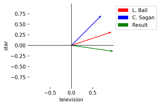
Subtraction
Description: Element-wise differences
Notation: \(A - B = (a_1 - b_1, a_2 - b_2, \dots, a_n - b_n)\)
Result: Vector of length \(n\)
C = A - B
plot_vectors(
    l2_norm(A),
    l2_norm(B),
    l2_norm(C),
    vector_labels = vector_labels + ["Result"],
    axis_labels = terms,
    colors = colors + ["green"]
)
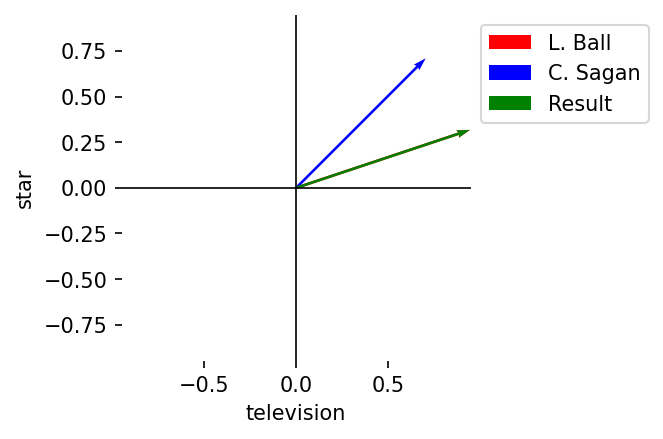
Multiplication, element-wise
Description: Element-wise products
Notation: \(A \circ B = (a_1 \cdot b_1, a_2 \cdot b_2, \dots, a_n \cdot b_n)\)
Result: Vector of length \(n\)
C = A * B
plot_vectors(
    l2_norm(A),
    l2_norm(B),
    l2_norm(C),
    vector_labels = vector_labels + ["Result"],
    axis_labels = terms,
    colors = colors + ["green"]
)
Multiplication, dot product
Description: The sum of the products
Notation: \(A \cdot B = \Sigma_{i=1}^{n} a_i \cdot b_i\)
Result: Single value (scalar)
A @ B
80
The dot product is one of the most important operations in modern machine learning. It measures the extent to which two vectors point in the same direction. If the dot product is positive, the angle between two vectors is under 90 degrees. This means they point somewhat in the same direction. If it is negative, they point in opposite directions. And when the dot product is zero, the vectors are perpendicular.
6.3. Cosine Similarity#
Recall that, initially, we wanted to understand how similar two vectors are. We can do so with the dot product. The dot product allows us to derive a measure of how similar two vectors are in their orientation in vector space by considering the angle formed between them. This measure is called cosine similarity, and it is a quintessential method for working in semantic space.
We express it as follows:
Where:
\(cos \theta\): cosine of the angle \(\theta\)
\(A \cdot B\): dot product of A and B
\(||A||||B||\): the product of A and B’s magnitudes
The denominator is a normalization operation, similar in nature to L2 normalization. It helps control for magnitude variance between vectors, which is important when documents are very different in length.
The function below derives a cosine similarity score for two vectors.
def calculate_cosine_similarity(A, B):
    """Calculate cosine similarity between two vectors.

    Parameters
    ----------
    A : np.ndarray
        First vector
    B : np.ndarray
        Second vector

    Returns
    -------
    cos_sim : float
        Cosine similarity of A and B
    """
    dot = A @ B
    norm_by = np.linalg.norm(A) * np.linalg.norm(B)
    cos_sim = dot / norm_by

    return np.round(cos_sim, 4)
Scores are between \([-1, 1]\), where:
\(1\): same orientation; perfect similarity
\(0\): orthogonal vectors; vectors have nothing in common
\(-1\): opposite orientation; vectors are the opposite of one another
Here’s A and A:
calculate_cosine_similarity(A, A)
1.0
A and B:
calculate_cosine_similarity(A, B)
0.8944
And A and its opposite:
calculate_cosine_similarity(A, -A)
-1.0
6.3.1. Document similarity#
Typically, however, you’d just use the scikit-learn implementation. It
returns a square matrix comparing each vector with every other vector in the
input. Below, we run it across our DTM.
doc_sim = cosine_similarity(dtm)
doc_sim = pd.DataFrame(doc_sim, columns = dtm.index, index = dtm.index)
doc_sim.head()
| Ada Lovelace | Robert E Lee | Andrew Johnson | Bedford Forrest | Lucretia Mott | Charles Darwin | Ulysses Grant | Mary Ewing Outerbridge | Emma Lazarus | Louisa M Alcott | ... | Bella Abzug | Fred W Friendly | Frank Sinatra | Hassan II | Iris Murdoch | King Hussein | Pierre Trudeau | Elliot Richardson | Charles M Schulz | Karen Sparck Jones | |
|---|---|---|---|---|---|---|---|---|---|---|---|---|---|---|---|---|---|---|---|---|---|
| Ada Lovelace | 1.000000 | 0.072500 | 0.095733 | 0.101333 | 0.091677 | 0.141985 | 0.170934 | 0.087086 | 0.140926 | 0.130201 | ... | 0.157298 | 0.116398 | 0.099424 | 0.108706 | 0.194042 | 0.102954 | 0.131275 | 0.120062 | 0.135016 | 0.289609 |
| Robert E Lee | 0.072500 | 1.000000 | 0.250310 | 0.292756 | 0.084679 | 0.119690 | 0.487814 | 0.093315 | 0.124351 | 0.129774 | ... | 0.121218 | 0.101031 | 0.104586 | 0.161621 | 0.125416 | 0.108918 | 0.135583 | 0.167889 | 0.088386 | 0.076981 |
| Andrew Johnson | 0.095733 | 0.250310 | 1.000000 | 0.214493 | 0.146720 | 0.181105 | 0.457404 | 0.148732 | 0.145326 | 0.154563 | ... | 0.264893 | 0.156056 | 0.165122 | 0.231702 | 0.160823 | 0.151998 | 0.225098 | 0.281469 | 0.148176 | 0.121830 |
| Bedford Forrest | 0.101333 | 0.292756 | 0.214493 | 1.000000 | 0.090199 | 0.155993 | 0.385671 | 0.065007 | 0.129868 | 0.130259 | ... | 0.139353 | 0.124977 | 0.114385 | 0.159466 | 0.129266 | 0.115831 | 0.132275 | 0.108845 | 0.108885 | 0.098397 |
| Lucretia Mott | 0.091677 | 0.084679 | 0.146720 | 0.090199 | 1.000000 | 0.161976 | 0.129401 | 0.100451 | 0.130107 | 0.205686 | ... | 0.155760 | 0.075647 | 0.151797 | 0.133952 | 0.139900 | 0.063735 | 0.148130 | 0.118926 | 0.100889 | 0.118720 |
5 rows × 379 columns
Let’s look at some examples. Below, we define a function to query for a document’s nearest neighbors. That is, we look for which documents are closest to that document in the vector space.
def k_nearest_neighbors(query, similarities, k = 10):
    """Find the k-nearest neighbors for a query.

    Parameters
    ----------
    query : str
        Index name for the query vector
    similarities : pd.DataFrame
        Cosine similarities to query
    k : int
        Number of neighbors to return

    Returns
    -------
    output : list[tuple]
        Neighbors and their scores
    """
    neighbors = similarities[query].nlargest(k)
    neighbors, scores = neighbors.index, np.round(neighbors.values, 3)
    output = [(neighbor, score) for neighbor, score in zip(neighbors, scores)]

    return output
k = 5
for name in ("Miles Davis", "Eleanor Roosevelt", "Willa Cather"):
    neighbors = k_nearest_neighbors(name, doc_sim, k = k)
    table = tabulate(neighbors, headers = ["Name", "Score"])
    print(table, end = "\n\n")
Name               Score
---------------  -------
Miles Davis        1
Sammy Davis Jr     0.458
Thelonious Monk    0.383
Dizzy Gillespie    0.382
Coleman Hawkins    0.344

Name                      Score
----------------------  -------
Eleanor Roosevelt         1
FDR                       0.62
Jacqueline Kennedy        0.434
Elizabeth Cady Stanton    0.427
Anne O Hare McCormick     0.423

Name                 Score
-----------------  -------
Willa Cather         1
Edith Wharton        0.437
Truman Capote        0.428
Marjorie Rawlings    0.409
Scott Fitzgerald     0.396
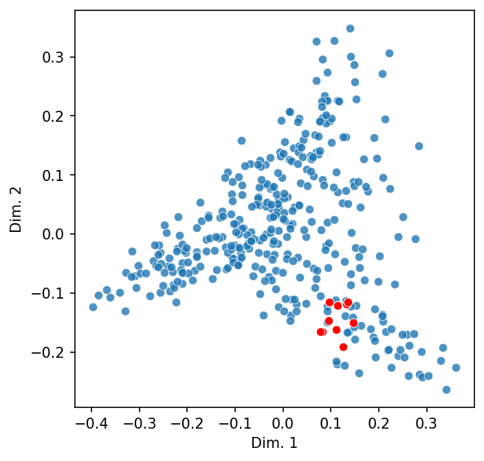
Does this conform to what we see in the scatter plot of documents?
names = doc_sim["Miles Davis"].nlargest(10).index
highlight = [dtm.index.get_loc(name) for name in names]
scatter_2d(dtm, highlight = highlight)
6.3.2. Token similarity#
All of the above applies to tokens as well. Transpose the DTM and you can derive cosine similarity scores between tokens.
token_sim = cosine_similarity(dtm.T)
token_sim = pd.DataFrame(token_sim, columns = dtm.columns, index = dtm.columns)
token_sim.sample(5)
| aachen | aahs | aane | aarau | aaron | aau | aaugh | aayega | aba | ababa | ... | zrathustra | zuber | zuker | zukor | zukors | zula | zululand | zurich | zvai | zwilich | |
|---|---|---|---|---|---|---|---|---|---|---|---|---|---|---|---|---|---|---|---|---|---|
| filter | 0.0 | 0.0 | 0.0 | 0.0 | 0.000000 | 0.0 | 0.0 | 0.0 | 0.0 | 0.0 | ... | 0.0 | 0.0 | 0.0 | 0.0 | 0.0 | 0.0 | 0.0 | 0.000000 | 0.0 | 0.0 |
| respective | 0.0 | 0.0 | 0.0 | 0.0 | 0.000000 | 0.0 | 0.0 | 0.0 | 0.0 | 0.0 | ... | 0.0 | 0.0 | 0.0 | 0.0 | 0.0 | 0.0 | 0.0 | 0.000000 | 0.0 | 0.0 |
| decorate | 0.0 | 0.0 | 0.0 | 0.0 | 0.140028 | 0.0 | 0.0 | 0.0 | 0.0 | 0.0 | ... | 0.0 | 0.0 | 0.0 | 0.0 | 0.0 | 0.0 | 0.0 | 0.022233 | 0.0 | 0.0 |
| fontainebleau | 0.0 | 0.0 | 0.0 | 0.0 | 0.000000 | 0.0 | 0.0 | 0.0 | 0.0 | 0.0 | ... | 0.0 | 0.0 | 0.0 | 0.0 | 0.0 | 0.0 | 0.0 | 0.000000 | 0.0 | 0.0 |
| quinn | 0.0 | 0.0 | 0.0 | 0.0 | 0.000000 | 0.0 | 0.0 | 0.0 | 0.0 | 0.0 | ... | 0.0 | 0.0 | 0.0 | 0.0 | 0.0 | 0.0 | 0.0 | 0.000000 | 0.0 | 0.0 |
5 rows × 31165 columns
Similar token listings:
k = 5
for token in ("music", "politics", "country", "royal"):
    neighbors = k_nearest_neighbors(token, token_sim, k = k)
    table = tabulate(neighbors, headers = ["Token", "Score"])
    print(table, end = "\n\n")
Token        Score
---------  -------
music        1
musical      0.738
piano        0.721
orchestra    0.701
musician     0.672

Token         Score
----------  -------
politics      1
democrats     0.693
democratic    0.669
political     0.652
campaign      0.647

Token      Score
-------  -------
country    1
time       0.773
people     0.77
great      0.757
end        0.757

Token      Score
-------  -------
royal      1
prince     0.862
osborne    0.853
coburg     0.85
saxe       0.85
We can also project these vectors into a two-dimensional space. The code below extracts the top-10 nearest tokens for a query token, samples the cosine similarities, adds the two together into a single DataFrame, and plots them. Note that we turn off normalization; cosine similarity is already normed.
# Get the subset, then sample
subset = token_sim["royal"].nlargest(10).index
sample = token_sim.sample(500)
sample = sample[~sample.index.isin(subset)]

# Make the DataFrame for plotting
to_plot = pd.concat([token_sim.loc[subset], sample])
highlight = [to_plot.index.get_loc(name) for name in subset]

# Plot
scatter_2d(to_plot, norm = False, highlight = highlight)
Technically, one could call these vectors definitions of each token. But they aren’t very good definitions—for a number of reasons, the first of which is that the only data we have to create these vectors comes from a small corpus of obituaries. We’d need a much larger corpus to generalize our token representations to a point where these vectors might reflect semantics as we understand it.
6.4. Word Embeddings#
Whence word embeddings. These vectors are the result of single-layer neural network training on millions, or even billions, of tokens. Networks will differ slightly in their architectures, but all are trained on co-occurrence tabulations, that is, the number of times a token appears alongside a set of tokens. The result: every token in the training data is embedded in a continuous vector space of many dimensions.
The two most common word embedding methods are Word2Vec and GloVe. The former uses a smaller window size of co-occurrences for a token, while the latter uses global co-occurrence values. Take a look at Jay Alammar’s Illustrated Word2Vec for a detailed walk-through of how these models are trained.
Below, we will use a 200-dimension version of GloVe, which continues
to be made available by the Stanford NLP group. It has been trained on a 2014
dump of Wikipedia and Gigaword 5. We define a custom class,
WordEmbeddings, to work with these vectors. Why do this? Word embeddings of
this kind have fallen out of favor by researchers and developers, and the
libraries that used to support embeddings have gone into maintenance-only mode.
class WordEmbeddings:
    """A minimal wrapper for Word2Vec-style embeddings.

    Loosely based on the Gensim wrapper: https://radimrehurek.com/gensim.
    """
    def __init__(self, path):
        """Initialize the embeddings.

        Parameters
        ----------
        path : str or Path
            Path to the embeddings parquet file
        """
        # Load the data and store some metadata about the vocabulary
        self.embeddings = pd.read_parquet(path)
        self.vocab = self.embeddings.index.tolist()
        self.vocab_size = len(self.vocab)

        # Fit a nearest neighbors graph using cosine similarity
        self.neighbors = NearestNeighbors(
            metric = "cosine", n_neighbors = len(self), n_jobs = -1
        )
        self.neighbors.fit(self.embeddings)

    def __len__(self):
        """Define a length for the embeddings."""
        return self.vocab_size

    def __getitem__(self, key):
        """Index the embeddings to retrieve a vector.

        Parameters
        ----------
        key : str
            Index key

        Returns
        -------
        vector : np.ndarray
            The vector
        """
        if key not in self.vocab:
            raise KeyError(f"{key} not in vocabulary.")

        return np.array(self.embeddings.loc[key])

    def similarity(self, source, target):
        """Find the similarity between two tokens.

        Parameters
        ----------
        source : str
            Source token
        target : str
            Target token

        Returns
        -------
        score : float
            Similarity score
        """
        # Query the neighbors graph to find the distances between it and all
        # other vectors
        query = self[source]
        distances = self.neighbors.kneighbors_graph([query], mode = "distance")
        distances = distances.toarray().squeeze(0)

        # Shift the distances to similarities
        similarities = 1 - distances

        # Return the target token's similarity using by indexing the
        # similarities
        idx = self.vocab.index(target)

        return similarities[idx]

    def most_similar(self, query, k = 1):
        """Find the k-most similar tokens to a query vector.

        Parameters
        ----------
        query : str or np.ndarray
            A query string or vector
        k : int
            Number of neighbors to return

        Returns
        -------
        output : list[tuple]
            Nearest tokens and their similarity scores
        """
        # If passed a string, get the vector
        if isinstance(query, str):
            query = self[query]

        # Query the nearest neighbor graph. This returns the index positions
        # for the top-k most similar tokens and the distance values for each of
        # those tokens
        distances, knn = self.neighbors.kneighbors([query], n_neighbors = k)

        # Convert distances to similarities and squeeze out the extra
        # dimension. Then retrieve tokens (and squeeze out that dimension, too)
        similarities = (1 - distances).squeeze(0)
        tokens = self.embeddings.iloc[knn.squeeze(0)].index

        # Pair the tokens with the similarities
        output = [(tok, sim) for tok, sim in zip(tokens, similarities)]

        return output

    def analogize(self, this = "", to_that = "", as_this = "", k = 1):
        """Perform an analogy and return the result's k-most similar neighbors.

        Parameters
        ----------
        this : str
            Analogy's source
        to_that : str
            Source's complement
        as_this : str
            Analogy's target
        k : int
            Number of neighbors to return

        Returns
        -------
        output : list[tuple]
            Nearest tokens and their similarity scores
        """
        # Get the vectors for input terms
        this, to_that, as_this = self[this], self[to_that], self[as_this]

        # Subtract the analogy's source from the analogy's target to capture
        # the relationship between the two (that is, their difference). Then,
        # apply this relationship to the source's complement via addition
        is_to_what = (as_this - this) + to_that

        # Get the most similar tokens to this new vector
        return self.most_similar(is_to_what, k)
With the wrapper defined, we load the embeddings.
glove = WordEmbeddings("data/models/glove.6B.200d.parquet")
n_vocab, n_dim = glove.embeddings.shape
print(f"Embeddings size and shape: {n_vocab:,} vectors, {n_dim} dimensions")
Embeddings size and shape: 400,000 vectors, 200 dimensions
And here’s an example embedding:
glove["book"]
array([-2.0744e-01,  4.1585e-01,  8.1915e-02,  5.8763e-02,  2.2087e-01,
        9.7051e-02, -4.2692e-01, -5.0030e-02,  3.1870e-01, -3.0463e-01,
        2.4791e-01,  5.6221e-01, -1.1726e-01,  3.1970e-01,  5.2722e-01,
        2.6074e-02, -3.6409e-01,  4.1153e-01, -7.6841e-01,  1.0559e-01,
        7.7134e-01,  2.3773e+00,  2.4155e-01, -1.1650e-01, -4.8823e-02,
        2.4152e-01, -2.0366e-01, -6.7341e-03, -7.4826e-02, -1.3317e-01,
       -4.3025e-01,  7.2237e-01,  6.4573e-01, -1.7853e-01,  3.4218e-01,
        2.0579e-01, -2.6898e-01, -4.5916e-01,  6.5838e-01, -7.6909e-01,
       -1.3438e-02,  2.2939e-01, -5.8398e-01,  3.0186e-01,  6.7211e-05,
        8.9954e-02,  1.1644e+00,  2.0050e-01,  8.2978e-02,  4.4839e-01,
       -3.2783e-01,  2.0404e-02,  5.9874e-01, -8.3142e-02,  1.8843e-01,
        1.2994e-01, -4.6333e-01,  4.8369e-01,  5.1809e-01,  3.5972e-02,
       -3.3864e-01,  5.1722e-01, -7.9211e-01, -4.8147e-01, -5.4961e-01,
       -3.3807e-01,  3.8443e-01,  3.7494e-01, -9.4575e-02,  4.6171e-01,
        1.4233e-02, -1.7931e-01,  1.7033e-01,  1.0492e-01,  3.2059e-01,
        1.8625e-01, -2.6142e-01, -2.5889e-01, -6.4226e-01, -1.4243e-01,
       -6.9478e-02,  3.6479e-01, -4.6202e-01,  3.9706e-01,  6.0458e-02,
       -5.4798e-02, -2.4068e-01, -1.5600e-01,  4.5201e-01, -6.4922e-01,
        1.4555e-01, -1.9309e-02,  2.3783e-01, -2.2749e-02,  1.9767e-01,
       -1.4548e-02,  1.4615e-01, -3.3319e-01, -5.0904e-01,  1.2364e-01,
       -2.4694e-01,  1.1290e-01,  7.1005e-01,  4.1276e-01,  5.3504e-02,
       -2.6021e-01, -1.2569e-01,  6.5647e-01, -4.7484e-01,  5.7874e-01,
        3.9066e-01, -3.3889e-01, -3.5945e-01, -2.6475e-01, -3.3406e-01,
       -1.9232e-02, -4.2046e-01,  6.1108e-01, -7.2916e-01, -2.7222e-01,
        1.2946e-02,  5.2870e-01, -4.1545e-01, -8.4026e-01, -8.8573e-02,
        6.2217e-02,  5.9892e-01,  2.3597e-01,  2.6234e-01, -6.3584e-01,
       -2.8773e-01,  2.9159e-02, -2.5226e-01,  4.2811e-02,  2.6993e-01,
        1.2566e-01, -1.2526e-01, -1.8764e-01, -3.6771e-01,  1.6834e-01,
        1.6387e-01, -9.1672e-02,  9.8863e-02,  2.2640e-01,  7.9722e-01,
       -1.2103e-01,  3.6880e-01, -9.5826e-01, -2.8817e-01,  1.4173e-01,
        5.4916e-01,  3.0036e-01, -6.5198e-01, -4.8353e-01,  5.2975e-01,
        3.4400e-01, -2.5168e-01, -2.5082e-01,  4.1813e-01, -4.3527e-02,
        3.8635e-01,  3.1218e-02,  2.6251e-01,  2.4787e-01,  7.2785e-01,
       -8.0236e-01, -6.1127e-01, -7.6405e-01, -3.0026e-01,  2.4254e-01,
       -2.3853e-01,  2.0024e-01,  5.7175e-01,  1.8369e-01, -1.5088e-01,
        6.9597e-01, -7.7065e-01,  4.4209e-01,  2.5416e-01,  2.3234e-01,
        1.0590e+00,  1.7118e-01, -2.9142e-01,  1.1264e-02, -9.5082e-01,
       -1.1275e-01, -4.1507e-01, -1.6546e-01,  1.7465e-01,  6.6374e-02,
       -4.1581e-01, -5.0738e-02,  4.2403e-01, -3.6238e-01,  6.1508e-01,
       -2.6538e-01, -4.6146e-01,  2.9840e-01,  5.1868e-01, -1.9248e-01])
6.4.1. Token similarity (redux)#
With the embeddings loaded, we query the same set of tokens from above to find their nearest neighbors.
k = 5
for token in ("music", "politics", "country", "royal"):
    neighbors = glove.most_similar(token, k = k)
    table = tabulate(neighbors, headers = ["Token", "Score"])
    print(table, end = "\n\n")
Token         Score
---------  --------
music      1
musical    0.733881
songs      0.725357
pop        0.690601
musicians  0.687654
Token           Score
-----------  --------
politics     1
political    0.767441
politicians  0.623498
religion     0.604117
liberal      0.59728
Token         Score
---------  --------
country    1
nation     0.81192
countries  0.692018
has        0.682141
now        0.66038
Token        Score
--------  --------
royal     1
queen     0.607112
imperial  0.606977
british   0.573261
palace    0.562962
Some listings, like the one for “music,” are fairly comparable, but listings for “country” and “royal” are more general.
To get the least similar token, query for all tokens and then select the last element. You may think this would be a token’s antonym.
glove.most_similar("good", k = len(glove))[-1]
('cw96', -0.6553233434020003)
Here, semantics and vector spaces diverge. The vector for the above token is in the opposite direction of the one for “good,” but that doesn’t line up with semantic opposition. In fact, the token we’d likely expect, “evil,” is relatively similar to “good.”
glove.similarity("good", "evil")
0.33780358010030886
Why is this? Since word embeddings are trained on co-occurrence data, tokens that appear in similar contexts will be more similar in a mathematical sense. We often speak of “good” and “evil” in interchangeable ways.
It’s important to keep this in mind for considerations of bias. Because embeddings reflect the interchangeability of tokens, they can reinforce negative, even harmful patterns in their training data.
k = 10
for token in ("doctor", "nurse"):
    neighbors = glove.most_similar(token, k = k)
    table = tabulate(neighbors, headers = ["Token", "Score"])
    print(table, end = "\n\n")
Token         Score
---------  --------
doctor     1
physician  0.736021
doctors    0.672406
surgeon    0.655147
dr.        0.652498
nurse      0.651449
medical    0.648189
hospital   0.63638
patient    0.619159
dentist    0.584747
Token           Score
-----------  --------
nurse        1
nurses       0.714051
doctor       0.651449
nursing      0.626938
midwife      0.614592
anesthetist  0.610603
physician    0.610359
hospital     0.609222
mother       0.586503
therapist    0.580488
6.4.2. Concept modeling#
Recall the vector operations we discussed above. We can perform these operations on word embeddings (since embeddings are vectors), and doing so provides a way to explore semantic space. One way to think about modeling concepts, for example, is by adding two vectors together. We’d expect the nearest neighbors of the resultant vector to reflect the concept we’ve tried to build.
The dictionary below has keys for concepts. Its tuples are the two vectors we’ll add together to create that concept.
concepts = {
    "beach": ("sand", "ocean"),
    "hotel": ("vacation", "room"),
    "airplane": ("air", "car")
}
Let’s iterate through the concepts.
k = 10
for concept in concepts:
    # Build the concept by adding the two component vectors
    A, B = concepts[concept]
    vector = glove[A] + glove[B]

    # Query the embeddings, print the results
    neighbors = glove.most_similar(vector, k = k)
    table = tabulate(neighbors, headers = ["Token", "Score"])
    print("Target:", concept, end = "\n\n")
    print(table, end = "\n\n")
Target: beach

Token       Score
-------  --------
sand     0.845458
ocean    0.845268
sea      0.687682
beaches  0.667521
waters   0.664894
coastal  0.632485
water    0.618701
coast    0.604373
dunes    0.599333
surface  0.597545
Target: hotel

Token         Score
---------  --------
vacation   0.82346
room       0.810719
rooms      0.704233
bedroom    0.658199
hotel      0.647865
dining     0.634925
stay       0.617807
apartment  0.616495
staying    0.615182
home       0.606009
Target: airplane

Token         Score
---------  --------
air        0.827957
car        0.810086
vehicle    0.719382
cars       0.671697
truck      0.645963
vehicles   0.637166
passenger  0.625993
aircraft   0.62482
jet        0.618584
airplane   0.610344
The expected concepts aren’t the top-most tokens for each result, but they’re in the top 10.
6.4.3. Analogies#
Most famously, word embeddings enable quasi-logical reasoning. Whereas synonym/antonym pairs do not map to vector operations, certain analogies do—or, sometimes they do. To construct these analogies, we define a relationship between a source and a target word by subtracting the vector for the former from the latter. Then, we add the source’s complement to the result. As above, the nearest neighbors for this new vector should reflect analogical reasoning.
Below: “Strong is to stronger what clear is to X?”.
k = 10
similarities = glove.analogize(
    this = "strong", to_that = "stronger", as_this = "clear", k = k
)
table = tabulate(similarities, headers = ["Token", "Score"])
print(table)
Token        Score
--------  --------
clear     0.707581
easier    0.635169
clearer   0.62249
stronger  0.609107
should    0.601482
harder    0.59936
better    0.59212
sooner    0.580909
must      0.57448
need      0.573058
“Paris is to France what Berlin is to X?”
k = 10
similarities = glove.analogize(
    this = "paris", to_that = "france", as_this = "berlin", k = k
)
table = tabulate(similarities, headers = ["Token", "Score"])
print(table)
Token       Score
-------  --------
germany  0.832399
berlin   0.678563
german   0.672207
france   0.62612
austria  0.616403
poland   0.59143
germans  0.575792
belgium  0.557132
britain  0.553339
spain    0.538451
Let’s plot the above example in two dimensions to demonstrate this.
# Get the embeddings
paris, france = glove["paris"], glove["france"]
berlin, germany = glove["berlin"], glove["germany"]

# Create a target and stack the five vectors
target = (berlin - paris) + france
stacked = np.vstack([paris, france, berlin, germany, target])

# Plot
scatter_2d(stacked, norm = False, highlight = [4], figsize = (3, 3))
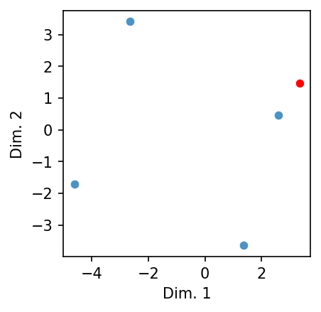
See how the target (in red) forms a perfect square with the other terms of the analogy? And its nearest neighbor is the vector we’d expect to find. That said: note that the latter does not form a perfect square. Analogizing in this manner fudges things.
Consider the following: “Arm is to hand what leg is to X?”
k = 10
similarities = glove.analogize(
    this = "arm", to_that = "hand", as_this = "leg", k = k
)
table = tabulate(similarities, headers = ["Token", "Score"])
print(table)
Token        Score
--------  --------
leg       0.763518
hand      0.606446
final     0.538706
legs      0.533707
table     0.515848
saturday  0.51571
round     0.512425
match     0.509738
draw      0.507376
second    0.501668
We’d expect “foot” but no such luck.
6.5. Part-of-Speech Disambiguation#
Clearly these embeddings pick up at least some information about semantics. But it’s challenging to identify where this information lies in the embeddings: sequences of positive and negative numbers don’t tell us much on their own. Let’s see if we can design an experiment to make these numbers more interpretable.
The following constructs a method for determining the part-of-speech (POS) of a vector. Using embeddings for POS-tagged WordNet lemmas, we train a classifier to make this determination.
6.5.1. Data preparation#
First, we load the embeddings for our WordNet tokens.
wordnet = pd.read_parquet(
    "data/datasets/wordnet_embeddings_glove.6B.200d.parquet"
)
Words can have more than one POS tag.
wordnet.loc[("good", slice(None))]
| 0 | 1 | 2 | 3 | 4 | 5 | 6 | 7 | 8 | 9 | ... | 190 | 191 | 192 | 193 | 194 | 195 | 196 | 197 | 198 | 199 | |
|---|---|---|---|---|---|---|---|---|---|---|---|---|---|---|---|---|---|---|---|---|---|
| label | |||||||||||||||||||||
| N | 0.51507 | 0.35596 | 0.1571 | -0.074075 | -0.25446 | -0.11357 | -0.49943 | -0.12626 | 0.38851 | 0.54204 | ... | -0.048109 | -0.38057 | -0.35258 | -0.006266 | 0.27227 | -0.16222 | -0.31979 | 0.14338 | -0.072859 | 0.17815 |
| A | 0.51507 | 0.35596 | 0.1571 | -0.074075 | -0.25446 | -0.11357 | -0.49943 | -0.12626 | 0.38851 | 0.54204 | ... | -0.048109 | -0.38057 | -0.35258 | -0.006266 | 0.27227 | -0.16222 | -0.31979 | 0.14338 | -0.072859 | 0.17815 |
2 rows × 200 columns
But the vectors are the same because static embeddings make no distinction in context-dependent determinations. We therefore drop duplicate vectors from our data. First though: we shuffle the rows. That will randomly distribute the POS tag distribution across all duplicated vectors (in other words, no one POS tag will unfairly benefit from dropping duplicates).
wordnet = wordnet.sample(frac = 1)
wordnet.drop_duplicates(inplace = True)
Now split the data into train/test sets. Our labels are the POS tags.
X = wordnet.values
y = wordnet.index.get_level_values(1)
X_train, X_test, y_train, y_test = train_test_split(
    X, y, test_size = 0.1, random_state = 357
)
Regardless of duplication, the tags themselves are fairly imbalanced.
tag_counts = pd.Series(y).value_counts()
tag_counts
label
N    27238
A    12475
V     4463
Name: count, dtype: int64
We derive a weighting to tell the model how often it should expect to see a tag.
class_weight = tag_counts / np.sum(tag_counts)
class_weight = {
    idx: np.round(class_weight[idx], 2) for idx in class_weight.index
}
class_weight
{'N': 0.62, 'A': 0.28, 'V': 0.1}
6.5.2. Fitting a logistic regression model#
We use a logistic regression model for this experiment. It models the probability that input data belongs to a specific class. In our case, input and classes are vectors and POS tags, respectively. For every dimension, or feature, in these vectors the model has a corresponding weight, or coefficient. Coefficients represent the change in the log-odds of the outcome for a one-unit change in the corresponding feature. Log-odds, or logits, are the logarithm of the odds of an event occurring (which is in turn the ratio of the probability of an event occurring to the probability of that event not occurring).
When training on data, the model multiplies features by their coefficients and sums them up to compute the log-odds of the outcome. This sum is used to obtain a probability for each class. The model adjusts its coefficients to increase the likelihood that the vector of features will be categorized with the correct label. At each step in the training process, a loss function (typically log loss) measures the difference between the predicted probabilities and the actual labels. The model uses this loss to update its coefficients in a way that reduces error.
Coefficients are represented as:
Where:
\(z\) is a vector of coefficients corresponding to each feature in the input \(x\)
\(\beta_0\) is the intercept, or bias term
\(\beta_nx_n\) is the product of the coefficient \(\beta_n\) for the \(n\)-th feature in the input \(x\)
Transforming \(z\) into a probability for each class uses the logistic, or sigmoid, function:
Where:
\(\hat{y}\) is the predicted probability
Which is the result of the sigmoid function \(\sigma(z)\)
\(\frac{1}{1 + e^{-z}}\) is sigmoid function formula
As with Naive Bayes, there’s no need to implement this ourselves when
scikit-learn can do it.
model = LogisticRegression(
    solver = "liblinear",
    C = 2.0,
    class_weight = class_weight,
    max_iter = 5_000,
    random_state = 357
)
model.fit(X_train, y_train)
LogisticRegression(C=2.0, class_weight={'A': 0.28, 'N': 0.62, 'V': 0.1},
                   max_iter=5000, random_state=357, solver='liblinear')
In a Jupyter environment, please rerun this cell to show the HTML representation or trust the notebook. On GitHub, the HTML representation is unable to render, please try loading this page with nbviewer.org.
LogisticRegression(C=2.0, class_weight={'A': 0.28, 'N': 0.62, 'V': 0.1},
                   max_iter=5000, random_state=357, solver='liblinear')
Let’s look at a classification report.
preds = model.predict(X_test)
report = classification_report(y_test, preds, target_names = model.classes_)
print(report)
              precision    recall  f1-score   support

           A       0.80      0.53      0.64      1248
           N       0.76      0.94      0.84      2713
           V       0.85      0.45      0.59       457

    accuracy                           0.77      4418
   macro avg       0.80      0.64      0.69      4418
weighted avg       0.78      0.77      0.76      4418
Not bad. For a such a simple model, it achieves decent accuracy, and the precision is relatively high. Recall suffers, however. This is likely due to the class imbalance.
6.5.3. Examining model coefficients#
Let’s extract the coefficients from the model. These represent the weightings on each dimension of the word vectors that adjust the associated values to be what the model expects for a certain class.
Positive coefficient: An increase in the feature value increases the log-odds of the classification outcome; the probability of a token belonging to the class increases
Negative coefficient: An increase in the feature value decreases the log-odds of the classification outcome; the probability of a token belonging to the class decreases
coef = pd.DataFrame(model.coef_.T, columns = model.classes_)
coef.head()
| A | N | V | |
|---|---|---|---|
| 0 | -0.217249 | 0.043046 | 0.029644 |
| 1 | -1.079837 | 0.653976 | 0.601929 |
| 2 | 0.282675 | -0.151351 | -0.225647 |
| 3 | 0.065292 | 0.022897 | -0.216423 |
| 4 | -0.488317 | 0.389618 | 0.334772 |
We’ll use this DataFrame in a moment, but for now let’s reformat to create a series of bar plots showing how each dimension of the embeddings interacts with the model’s coefficients.
coef_plot = coef.reset_index().rename(columns = {"index": "dimension"})
coef_plot = pd.melt(
    coef_plot,
    id_vars = "dimension",
    var_name = "POS",
    value_name = "coefficient"
)
Time to plot.
fig, axes = plt.subplots(3, 1, figsize = (15, 5), sharex = True, sharey = True)
for idx, pos in enumerate(model.classes_):
    subplot_data = coef_plot[coef_plot["POS"] == pos]
    g = sns.barplot(
        x = "dimension",
        y = "coefficient",
        data = coef_plot[coef_plot["POS"] == pos],
        ax = axes[idx]
    )
    g.set(ylabel = f"{pos} coefficient", xticklabels = [])

plt.suptitle("POS coefficients across word embedding dimensions")
plt.tight_layout()
plt.show()
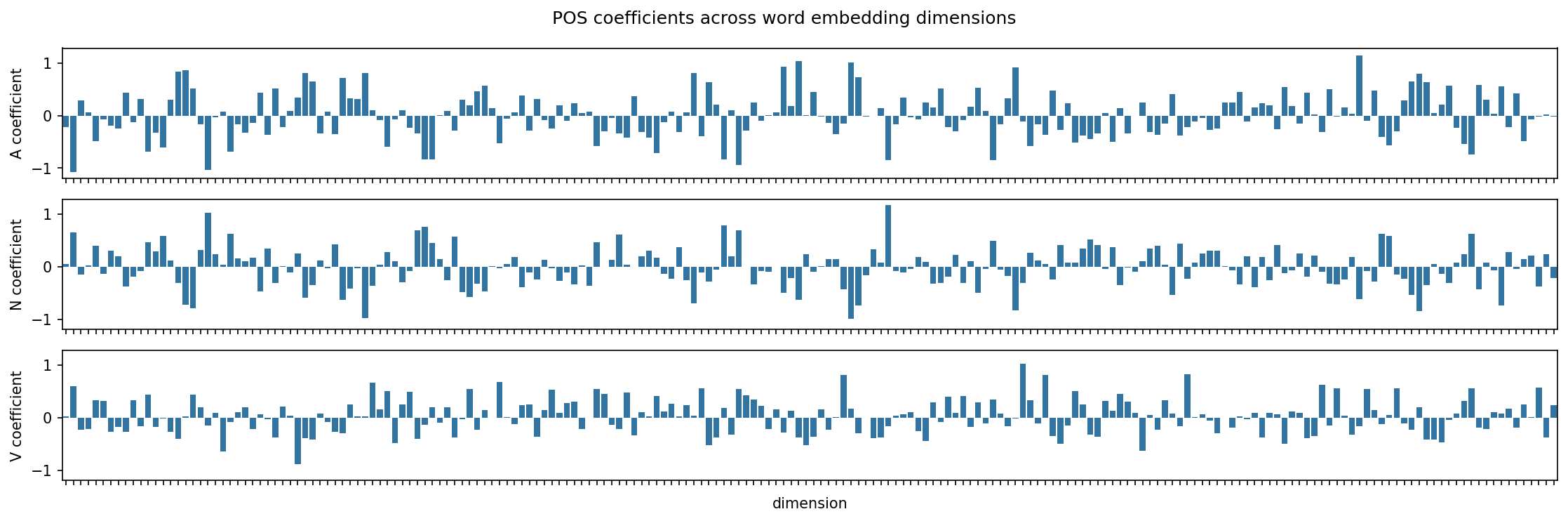
No one single dimension stands out as the indicator for a POS tag; rather, groups of dimensions determine POS tags. This is in part what we mean by a distributed representation. We can use recursive feature elimination to extract dimensions that are particularly important. This process fits our model on the embedding features and then evaluates the importance of each feature. Important features are those with high coefficients (absolute values). It then prunes out the least important features, refits the model, re-evaluates feature importance, and so on.
Use n_features_to_select to set the number of features you want. Supplying an
argument to step will determine how many features are pruned out at every
step.
selector = RFE(model, n_features_to_select = 10, step = 5)
selector.fit(X_train, y_train)
RFE(estimator=LogisticRegression(C=2.0,
                                 class_weight={'A': 0.28, 'N': 0.62, 'V': 0.1},
                                 max_iter=5000, random_state=357,
                                 solver='liblinear'),
    n_features_to_select=10, step=5)
In a Jupyter environment, please rerun this cell to show the HTML representation or trust the notebook. On GitHub, the HTML representation is unable to render, please try loading this page with nbviewer.org.
RFE(estimator=LogisticRegression(C=2.0,
                                 class_weight={'A': 0.28, 'N': 0.62, 'V': 0.1},
                                 max_iter=5000, random_state=357,
                                 solver='liblinear'),
n_features_to_select=10, step=5)LogisticRegression(C=2.0, class_weight={'A': 0.28, 'N': 0.62, 'V': 0.1},
max_iter=5000, random_state=357, solver='liblinear')LogisticRegression(C=2.0, class_weight={'A': 0.28, 'N': 0.62, 'V': 0.1},
max_iter=5000, random_state=357, solver='liblinear')Collect the dimension names from the feature selector and plot the corresponding coefficients.
important_features = selector.get_support(indices = True)
fig, ax = plt.subplots(figsize = (15, 5))
g = sns.barplot(
    x = "dimension",
    y = "coefficient",
    hue = "POS",
    palette = "tab10",
    data = coef_plot[coef_plot["dimension"].isin(important_features)],
    ax = ax

)
g.set(title = "Ten most important features for determining a POS tag")
sns.move_legend(ax, "upper left", bbox_to_anchor = (1, 1))
plt.show()
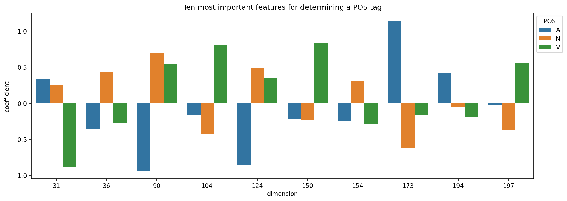
6.5.4. Tag associations#
If we multiply the vectors by the model coefficients, we can determine the degree to which each sample is associated with a POS tag. This will concretely ground the above graphs in specific tokens.
associations = np.dot(wordnet, coef)
associations = pd.DataFrame(
    associations, index = wordnet.index, columns = model.classes_
)
associations.sample(5)
| A | N | V | ||
|---|---|---|---|---|
| token | label | |||
| howitzer | N | 1.392822 | -0.143321 | -1.989826 |
| rationalize | V | -1.337992 | -2.817569 | 6.089466 |
| sound | V | 2.558355 | -2.366026 | -0.519853 |
| assimilatory | A | 1.559594 | -0.028936 | -2.082446 |
| bombard | V | -0.980726 | -2.586952 | 5.504883 |
Let’s look at some tokens. Below, we show tokens that are unambiguously one
kind of word or another. Using the .idxmax() method will return which column
has the highest coefficient.
inspect = ["colorless", "lion", "recline"]
associations.loc[(inspect, slice(None))].idxmax(axis = 1)
token      label
colorless  A        A
lion       N        N
recline    V        V
dtype: object
That seems to work pretty well! But let’s look at a word that can be more than one POS.
inspect = ["good", "goad", "great"]
associations.loc[(inspect, slice(None))].idxmax(axis = 1)
token  label
good   N        A
goad   V        V
great  N        N
dtype: object
Here we see the constraints of static embeddings. The coefficients for these words favor one POS over another, and that should make sense: the underlying embeddings make no distinction between two. One reason why our classifier doesn’t always perform well very likely has to do with this as well.
That said, getting class probabilities tells a slightly more encouraging story.
for token in inspect:
    vector = glove[token]
    probs = model.predict_proba([vector]).squeeze(0)

    print(f"Predictions for '{token}':")
    for idx, label in enumerate(model.classes_):
        print(f"  {label}: {probs[idx]:.2f}%")
Predictions for 'good':
  A: 0.34%
  N: 0.65%
  V: 0.01%
Predictions for 'goad':
  A: 0.03%
  N: 0.38%
  V: 0.59%
Predictions for 'great':
  A: 0.01%
  N: 0.99%
  V: 0.00%
The label with the second-highest probability tends to be for a token’s other POS tag.
6.5.5. Shifting vectors#
The above probabilities suggest that a token is somewhat like one POS and somewhat like another. On the one hand that conforms with how we understand POS tags to work; but on the other, it matches the additive nature of logistic regression: each set of coefficients indicates how much a given feature in the vector contributes to a particular class prediction. This property about coefficients also suggests a way to modify vectors so that they are more like one POS tag or another.
The function below does just that. It shifts the direction of a vector in vector space so that its orientation is more like a particular POS tag. How does it do so? With simple addition: we add the coefficients for our desired POS tag to the vector in question.
def shift_vector(vector, coef, glove = glove, k = 25):
    """Shift the direction of a vector by combining it with a coefficient.

    Parameters
    ----------
    vector : nd.ndarray
        The vector to shift
    coef : np.ndarray
        Coefficient vector
    glove : WordEmbeddings
        The word embeddings
    k : int
        Number of nearest neighbors to return

    Returns
    -------
    neighbors : list[tuple]
        The k-nearest neighbors for the original and shifted vectors
    """
    # Find the vector's k-nearest neighbors
    vector_knn = glove.most_similar(vector, k)

    # Now shift it by adding the coefficient. Then normalize and find the
    # k-nearest neighbors of this new vector
    shifted = vector + coef
    shifted /= np.linalg.norm(shifted)
    shifted_knn = glove.most_similar(shifted, k)

    # Extract the tokens and put them into a DataFrame
    neighbors = [
        (tok1, tok2) for (tok1, _), (tok2, _) in zip(vector_knn, shifted_knn)
    ]

    return neighbors
Let’s try this with a few tokens. Below, we make “dessert” more like an adjective.
shifted = shift_vector(glove["dessert"], coef["A"])
table = tabulate(shifted, headers = ["Original", "Shifted"])
print(table)
Original    Shifted
----------  -----------
dessert     dessert
desserts    desserts
delicious   delicious
appetizer   appetizer
cake        tasting
chocolate   tasty
appetizers  appetizers
cakes       dishes
salad       pastries
dish        cakes
salads      salads
tasting     savory
dishes      baked
pastries    concoctions
baked       wines
menu        concoction
pudding     flavors
entree      delectable
cream       dish
wine        chocolate
meal        recipes
sorbet      confection
cookies     cake
flavors     pies
tiramisu    meals
How about “desert”?
shifted = shift_vector(glove["desert"], coef["A"])
table = tabulate(shifted, headers = ["Original", "Shifted"])
print(table)
Original     Shifted
-----------  ------------
desert       desert
deserts      deserts
arid         arid
mojave       desolate
mountains    barren
chihuahuan   terrain
sonoran      coastal
namib        mojave
barren       mountains
gobi         mountainous
desolate     rugged
coastal      inhospitable
sahara       vast
negev        sonoran
dunes        remote
taklamakan   areas
terrain      populated
southern     chihuahuan
mountain     oases
cholistan    dunes
plains       namib
vast         surrounded
mountainous  expanse
taklimakan   beaches
remote       parched
Now make “language” more like a verb.
shifted = shift_vector(glove["language"], coef["V"])
table = tabulate(shifted, headers = ["Original", "Shifted"])
print(table)
Original     Shifted
-----------  -----------
language     language
languages    languages
arabic       speak
word         arabic
english      word
spoken       english
words        words
speak        translate
vocabulary   learn
meaning      teach
translation  write
speaking     describe
literature   meaning
dialect      understand
bilingual    vocabulary
hindi        spoken
writing      refer
urdu         hindi
dialects     translation
programming  dialects
text         speakers
hebrew       dialect
speakers     read
learning     define
means        bilingual
The modifications here are subtle, but they do exist: while the top-most similar tokens tend to be the same between the original and shifted vectors, their ordering moves around, often in ways that conform to what you’d expect to see with the POS’s valences.
shifted = shift_vector(glove["drive"], coef["N"])
table = tabulate(shifted, headers = ["Original", "Shifted"])
print(table)
Original    Shifted
----------  ---------
drive       drive
drives      drives
drove       drove
driving     driving
driven      car
push        driven
turn        comes
car         goes
effort      vehicle
hard        push
off         stop
way         runs
run         end
back        off
end         driver
vehicle     wheel
go          a
trying      hard
stop        effort
pull        running
move        speed
attempt     another
just        back
cars        program
get         road