8. Bidirectional Encoder Representations from Transformers (BERT)#
This chapter demonstrates fine tuning with a BERT model, discussing data preparation, hyperparameter configurations, model training, and model evaluation. It then uses SHAP values to ground model predictions in concrete tokens.
Data: The University of Hamburg Language Technology Group’s Blurb Genre Collection, a large dataset of English book blurbs
Credits: Portions of this chapter are adapted from the UC Davis DataLab’s Natural Language Processing for Data Science
8.1. Preliminaries#
We will need several imports for this chapter.
import unicodedata
import torch
import numpy as np
import pandas as pd
from datasets import Dataset
from transformers import (
AutoTokenizer,
AutoModelForSequenceClassification,
DataCollatorWithPadding,
TrainingArguments,
Trainer,
EarlyStoppingCallback,
pipeline
)
import evaluate
from sklearn.metrics import classification_report, confusion_matrix
import shap
from nltk.corpus import stopwords
import matplotlib.pyplot as plt
import seaborn as sns
With imports finished, we load the data.
blurbs = pd.read_parquet("data/datasets/ltg_book_blurbs.parquet")
Currently the labels for this data are string representations of genres.
blurbs["d1"].sample(5).tolist()
['Politics',
'Graphic Novels & Manga',
'Romance',
'Romance',
'Mystery & Suspense']
We need to convert those strings into unique identifiers. In most cases, the
unique identifier is just an arbitrary number; we create them below by taking
the index position of a label in the .unique() output. Under the hood, the
model will use those numbers, but if we associate them in a dictionary with the
original strings, we can also have it display the original strings.
enumerated = list(enumerate(blurbs["d1"].unique()))
id2label = {idx: genre for idx, genre in enumerated}
label2id = {genre: idx for idx, genre in enumerated}
Use .replace() to remap the labels in the data.
blurbs["label"] = blurbs["d1"].replace(label2id)
How many unique labels are there?
num_labels = blurbs["label"].nunique()
print(num_labels, "unique labels")
10 unique labels
What is the distribution of labels like?
blurbs.value_counts("label")
label
0 1459
1 1459
2 1459
3 1459
4 1459
5 1459
6 1459
7 1459
8 1459
9 1459
Name: count, dtype: int64
With model-ready labels made, we create a Dataset. These objects work
directly with the Hugging Face training pipeline to handle batch processing and
other such optimizations in an automatic fashion. They also allow you to
interface directly with Hugging Face’s cloud-hosted data, though we will only
use local data for this fine-tuning run.
We only need two columns from our original DataFrame: the text and its label.
dataset = Dataset.from_pandas(blurbs[["text", "label"]])
dataset
Dataset({
features: ['text', 'label'],
num_rows: 14590
})
Finally, we load a model to fine-tune. This works just like we did earlier,
though the AutoModelForSequenceClassification object expects to have an
argument that specifies how many labels you want to train your model to
recognize.
ckpt = "bert-base-uncased"
tokenizer = AutoTokenizer.from_pretrained(ckpt)
model = AutoModelForSequenceClassification.from_pretrained(
ckpt, num_labels = num_labels
)
Don’t forget to associate the label mappings!
model.config.id2label = id2label
model.config.label2id = label2id
8.2. Data Preparation#
Data preparation will also work very much like past modeling tasks. Below, we define a simple tokenization function. This just wraps the usual functionality that a tokenizer would do, but keeping that functionality stored in a custom wrapper like this allows us to cast, or map, that function across the entire Dataset all at once.
def tokenize(examples):
"""Tokenize strings.
Parameters
----------
examples : dict
Batch of texts
Returns
-------
tokenized : dict
Tokenized texts
"""
tokenized = tokenizer(examples["text"], truncation = True)
return tokenized
Now we split the data into separate train/test datasets…
split = dataset.train_test_split()
split
DatasetDict({
train: Dataset({
features: ['text', 'label'],
num_rows: 10942
})
test: Dataset({
features: ['text', 'label'],
num_rows: 3648
})
})
…and tokenize both with the function we’ve written. Note the batched
argument. It tells the Dataset to send batches of texts to the tokenizer at
once. That will greatly speed up the tokenization process.
trainset = split["train"].map(tokenize, batched = True)
testset = split["test"].map(tokenize, batched = True)
Tokenizing texts like this creates the usual output of token ids, attention masks, and so on:
trainset
Dataset({
features: ['text', 'label', 'input_ids', 'token_type_ids', 'attention_mask'],
num_rows: 10942
})
Recall from the last chapter that models require batches to have the same number of input features. If texts are shorter than the total feature size, we pad them and then tell the model to ignore that padding during processing. But there may be cases where an entire batch of texts is substantially padded because all those texts are short. It would be a waste of time and computing resources to process them with all that padding.
This is where the DataCollatorWithPadding comes in. During training it will
dynamically pad batches to the maximum feature size for a given batch. This
improves the efficiency of the training process.
data_collator = DataCollatorWithPadding(tokenizer = tokenizer)
8.3. Model Training#
With our data prepared, we move on to setting up the training process.
8.3.1. Logging metrics#
It’s helpful to monitor how a model is doing while it trains. The function below computes metrics when the model pauses to perform an evaluation. During evaluation, the model trainer will call this function, calculate the scores, and display the results.
The scores are simple ones: accuracy and F1. To calculate them, we use the
evaluate package, which is part of the Hugging Face ecosystem.
accuracy_metric = evaluate.load("accuracy")
f1_metric = evaluate.load("f1")
def compute_metrics(evaluations):
"""Compute metrics for a set of predictions.
Parameters
----------
evaluations : tuple
Model logits/label for each text and texts' true labels
Returns
-------
scores : dict
The metric scores
"""
# Split the model logits from the true labels
logits, references = evaluations
# Find the model prediction with the maximum value
predictions = np.argmax(logits, axis = 1)
# Calculate the scores
accuracy = accuracy_metric.compute(
predictions = predictions, references = references
)
f1 = f1_metric.compute(
predictions = predictions,
references = references,
average = "weighted"
)
# Wrap up the scores and return them for display during logging
scores = {"accuracy": accuracy["accuracy"], "f1": f1["f1"]}
return scores
8.3.2. Training hyperparameters#
There are a large number of hyperparameters to set when training a model. Some of them are very general, some extremely granular. This section walks through some of the most common ones you will find yourself adjusting.
First: epochs. The number of epochs refers to the number of times a model passes over the entire dataset. Big models train for dozens, even hundreds of epochs, but ours is small enough that we only need a few
num_train_epochs = 15
Training is broken up into individual steps. A step refers to a single update of the model’s parameters, and each step processes one batch of data. Batch size determines how many samples a model processes in each step.
Batch size can greatly influence training performance. Larger batch sizes tend to produce models that struggle to generalize (see here for a discussion of why). You would think, then, that you would want to have very small batches. But that would be an enormous trade-off in resources, because small batches take longer to train. So, setting the batch size ends up being a matter of balancing these two needs.
A good starting point for batch sizes is 32-64. Note that models have separate size specifications for the training batches and the evaluation batches. It’s a good idea to keep the latter set to a smaller size, for the very reason about measuring model generalization above.
per_device_train_batch_size = 32
per_device_eval_batch_size = 8
Learning rate controls how quickly your model fits to the data. One of the most important hyperparameters, it is the amount by which the model updates its weights at each step. Learning rates are often values between 0.0 and 1.0. Large learning rates will speed up training but lead to sub-optimally fitted models; smaller ones require more steps to fit the model but tend to produce a better fit (though there are cases where they can force models to become stuck in local minima).
Hugging Face’s trainer defaults to 5e-5 (or 0.00005). That’s a good starting
point. A good lower bound is 2e-5; we will use 3e-5.
learning_rate = 3e-5
Early in training, models can make fairly substantial errors. Adjusting for those errors by updating parameters is the whole point of training, but making adjustments too quickly could lead to a sub-optimally fitted model. Warm up steps help stabilize a model’s final parameters by gradually increasing the learning rate over a set number of steps.
It’s typically a good idea to use 10% of your total training steps as the step size for warm up.
warmup_steps = (len(trainset) / per_device_train_batch_size) * num_train_epochs
warmup_steps = round(warmup_steps * 0.1)
print("Number of warm up steps:", warmup_steps)
Number of warm up steps: 513
Weight decay helps prevent overfitted models by keeping model weights from
growing too large. It’s a penalty value added to the loss function. A good
range for this value is 1e-5 - 1e-2; use a higher value for smaller
datasets and vice versa.
weight_decay = 1e-2
With our primary hyperparameters set, we specify them using a
TrainingArguments object. There are only a few other things to note about
initializing our TrainingArgumnts. Besides specifying an output directory and
logging steps, we specify when the model should evaluate itself (after every
epoch) and provide a criterion (loss) for selecting the best performing model
at the end of training.
training_args = TrainingArguments(
output_dir = "data/bert_blurb_classifier",
num_train_epochs = num_train_epochs,
per_device_train_batch_size = per_device_train_batch_size,
per_device_eval_batch_size = per_device_eval_batch_size,
learning_rate = learning_rate,
warmup_steps = warmup_steps,
weight_decay = weight_decay,
logging_steps = 100,
evaluation_strategy = "epoch",
save_strategy = "epoch",
load_best_model_at_end = True,
metric_for_best_model = "loss",
save_total_limit = 3,
push_to_hub = False
)
8.3.3. Model training#
Once all the above details are set, we initialize a Trainer and supply it
with everything we’ve created: the model and its tokenizer, the data collator,
training arguments, training and testing data, and the function for computing
metrics. The only thing we haven’t seen below is the EarlyStoppingCallback.
This combats overfitting. When the model doesn’t improve after some number of
epochs, we stop training.
trainer = Trainer(
model = model,
tokenizer = tokenizer,
data_collator = data_collator,
args = training_args,
train_dataset = trainset,
eval_dataset = testset,
compute_metrics = compute_metrics,
callbacks = [EarlyStoppingCallback(early_stopping_patience = 3)]
)
Time to train!
trainer.train()
Calling this method would quick off the training process, and you would see logging information as it runs. But for reasons of time and computing resources, the underlying code of this chapter won’t run a fully training loop. Instead, it will load a separately trained model for evaluation.
But before that, we show how to save the final model:
trainer.save_model("data/models/bert_blurb_classifier/final")
Saving the model will save all the pieces you need when using it later.
8.4. Model Evaluation#
We will evaluate the model in two ways, first by looking at classification accuracy, then token influence. To do this, let’s re-load our model and tokenizer. This time we specify the path to our local model.
fine_tuned = "data/models/bert_blurb_classifier/final"
tokenizer = AutoTokenizer.from_pretrained(fine_tuned)
model = AutoModelForSequenceClassification.from_pretrained(fine_tuned)
8.4.1. Using a pipeline#
While we could separately tokenize texts and feed them through the model, a
pipeline will take care of all this. All we need to do is specify what kind
of task our model has been trained to do.
classifier = pipeline(
"text-classification", model = model, tokenizer = tokenizer
)
Below, we put a single text through the pipeline. It will return the model’s
prediction and a confidence score in a list, which we unpack with ,=.
sample = blurbs.sample(1)
result ,= classifier(sample["text"].item())
What does the model think this text is?
print(f"Model label: {result["label"]} ({result["score"]:.2f}% conf.)")
Model label: Graphic Novels & Manga (0.98% conf.)
What is the actual label?
print("Actual label:", sample["d1"].item())
Actual label: Graphic Novels & Manga
Here are the top three labels for this text:
classifier(sample["text"].item(), top_k = 3)
[{'label': 'Graphic Novels & Manga', 'score': 0.975226640701294},
{'label': 'Children’s Middle Grade Books', 'score': 0.018488172441720963},
{'label': 'Arts & Entertainment', 'score': 0.0010197801748290658}]
Set top_k to None to return all scores.
classifier(sample["text"].item(), top_k = None)
[{'label': 'Graphic Novels & Manga', 'score': 0.975226640701294},
{'label': 'Children’s Middle Grade Books', 'score': 0.018488172441720963},
{'label': 'Arts & Entertainment', 'score': 0.0010197801748290658},
{'label': 'Mystery & Suspense', 'score': 0.000912792922463268},
{'label': 'Romance', 'score': 0.0008446528809145093},
{'label': 'Politics', 'score': 0.0008410510490648448},
{'label': 'Cooking', 'score': 0.0008091511554084718},
{'label': 'Religion & Philosophy', 'score': 0.0007690949714742601},
{'label': 'Biography & Memoir', 'score': 0.000678630021866411},
{'label': 'Literary Fiction', 'score': 0.00041002299985848367}]
Each of these scores are probabilities. Sum them together and you would get \(1.0\). When the model selects a label, it chooses the label with the highest probability. This selection strategy is known as argmax.
Where \(c\) is the assigned class because the probability \(P\) is highest of all possible classes.
8.4.2. Classification accuracy#
Let’s look at a broader sample of blurbs and appraise the model’s performance. Below, we take 250 blurbs and send them through the pipeline. Note that this will mix training/evaluation datasets, but for the purposes of demonstration, it’s okay to sample from our data generally.
sample_large = blurbs.sample(250)
predicted = classifier(sample_large["text"].tolist(), truncation = True)
Now, we access the predicted labels and compare them against the true labels
with classification_report().
y_true = sample_large["d1"].tolist()
y_pred = [prediction["label"] for prediction in predicted]
report = classification_report(y_true, y_pred, zero_division = 0.0)
print(report)
precision recall f1-score support
Arts & Entertainment 0.90 1.00 0.95 19
Biography & Memoir 0.87 0.80 0.83 25
Children’s Middle Grade Books 0.90 0.95 0.93 20
Cooking 1.00 1.00 1.00 26
Graphic Novels & Manga 1.00 0.96 0.98 23
Literary Fiction 0.87 0.83 0.85 24
Mystery & Suspense 0.96 0.92 0.94 24
Politics 0.96 0.88 0.92 26
Religion & Philosophy 0.91 1.00 0.95 29
Romance 0.91 0.94 0.93 34
accuracy 0.93 250
macro avg 0.93 0.93 0.93 250
weighted avg 0.93 0.93 0.93 250
Overall, these are pretty nice results. The F1 scores are fairly well balanced. Though it looks like the model struggles with classifying Biography & Memoir and Literary Fiction. But other genres, like Cooking and Romance, are just fine. We can use a confusion matrix to see which of these genres the model confuses with others.
confusion = confusion_matrix(y_true, y_pred)
confusion = pd.DataFrame(
confusion, columns = label2id.keys(), index = label2id.keys()
)
Plot the matrix as a heatmap:
plt.figure(figsize = (5, 5))
g = sns.heatmap(confusion, annot = True, cmap = "Blues")
g.set(ylabel = "True label", xlabel = "Predicted label")
plt.show()
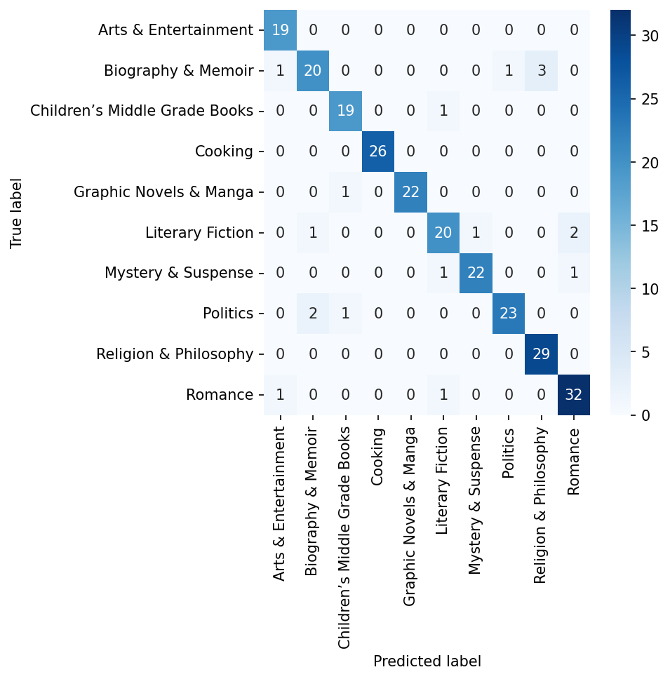
For this testing set, it looks like the model sometimes mis-classifies Biography & Memoir as Religion & Philosophy. Likewise, it sometimes assigns Politics to Biography & Memoir. Finally, there appears to be a little confusion between Literary Fiction and Romance.
Let’s look at some specific examples where the model is mistaken. First, we create a DataFrame.
inspection_df = pd.DataFrame({
"text": sample_large["text"].tolist(),
"label": y_true,
"pred": y_pred
})
We subset on mis-classifications.
mask = inspection_df["label"] != inspection_df["pred"]
wrong = inspection_df[mask]
Instances where the true label is Biography & Memoir but the model predicts Politics are especially revealing. These are often blurbs for memoirs written by political figures or by those who experienced significant political events.
wrong_doc = wrong.loc[
(wrong["label"] == "Biography & Memoir") & (wrong["pred"] == "Politics"),
"text"
].sample().item()
print(wrong_doc)
National Bestseller One of the Best Books of the Year: NPR, Harper’s BazaarJoan Didion has always kept notebooks—of overheard dialogue, interviews, drafts of essays, copies of articles. South and West gives us two extended excerpts from notebooks she kept in the 1970s; read together, they form a piercing view of the American political and cultural landscape. “Notes on the South” traces a road trip that she and her husband, John Gregory Dunne, took through Louisiana, Mississippi, and Alabama. Her acute observations about the small towns they pass through, her interviews with local figures, and their preoccupation with race, class, and heritage suggest a South largely unchanged today. “California Notes” began as an assignment from Rolling Stone on the Patty Hearst trial. Though Didion never wrote the piece, the time she spent watching the trial in San Francisco triggered thoughts about the West and her own upbringing in Sacramento. Here we not only see Didion’s signature irony and imagination in play, we’re also granted an illuminating glimpse into her mind and process.
That seems sensible enough. But right now, we only have two strategies for making sense of these mis-classifications: looking at the model’s label assignments or reading the texts ourselves. There’s no middle ground between high-level summary or low-level reading.
8.5. SHAP Values#
To bridge these two levels, we will turn to SHAP values. SHAP values provide a method of interpreting various machine learning models, including LLMs. Each one of these values represents how important a particular feature is for a model’s prediction. In the case of BERT, these features are tokens. Using SHAP values, we can rank how important each token in a blurb is. This, in short, provides us with a way to highlight what the model is paying attention to when it makes its decisions.
SHAP stands for “SHapley Additive exPlanations.” They are generalizations of the Shapley value, a concept from game theory developed by Lloyd Shapley. In a gaming scenario, a Shapley value describes how much a player contributes to an outcome vis-a-vis a subset, or coalition, of all players in the game. The process of deriving this value is detailed below:
Marginal contribution: The difference in the value of a coalition when a player is included versus when that player is excluded
Coalition: Any subset of the total number of players. A coalition’s value is the benefit that a coalition’s players achieve when they work together
Shapley value: This value is computed by calculating a player’s marginal contributions to all possible permutations of coalitions. The average of these contributions is the final value
In the context of machine learning, players are features in the data (tokens). A coalition of these features produces some value, computed by the model’s prediction function (e.g., argmax classification). SHAP values describe how much each feature contributes to the value produced by a coalition.
The formula for calculating SHAP (and Shapley) values is as follows:
Where:
\(\phi_i(v)\) is the SHAP value for player \(i\)
\(S\) is a subset of the set of all players \(N\) excluding player \(i\) \((N \setminus \{i\})\)
\(|S|\) is the number of players in subset \(S\)
\(|N|\) is the total number of players
\(v(S)\) is the value of a subset \(S\)
\(v(S \cup \{i\}) - v(S)\) is the marginal contribution of player \(i\) to subset \(S\)
8.5.1. Building an explainer#
Luckily, we needn’t calculate these values by hand; we can use the SHAP
library instead. The logic of this library is to wrap a machine learning model
with an Explainer, which, when called, will perform the above computations by
permuting all features in each blurb and measuring the difference those
permutations make for the final outcome.
We set up an Explainer below. It requires a few more defaults for the
pipeline objection, so we will re-initialize that as well.
classifier = pipeline(
"text-classification",
model = model,
tokenizer = tokenizer,
top_k = None,
truncation = True,
padding = True,
max_length = tokenizer.model_max_length
)
explainer = shap.Explainer(
classifier, output_names = list(model.config.id2label.values()), seed = 357
)
8.5.2. Individual values#
Let’s run our example from earlier through the Explainer. It may take a few
minutes on a CPU because this process must permute all possible token
coalitions.
explanation = explainer([sample["text"].item()])
The .base_values attribute contains expected values of the model’s
predictions for each class across the entire dataset. Their units are
probabilities.
explanation.base_values
array([[0.20567036, 0.05563394, 0.0600453 , 0.14713407, 0.02409829,
0.12062163, 0.08335671, 0.09201474, 0.10876061, 0.10266432]])
We align them with the labels like so:
example_base = pd.DataFrame(
explanation.base_values, columns = explanation.output_names
)
example_base
| Arts & Entertainment | Biography & Memoir | Children’s Middle Grade Books | Cooking | Graphic Novels & Manga | Literary Fiction | Mystery & Suspense | Politics | Religion & Philosophy | Romance | |
|---|---|---|---|---|---|---|---|---|---|---|
| 0 | 0.20567 | 0.055634 | 0.060045 | 0.147134 | 0.024098 | 0.120622 | 0.083357 | 0.092015 | 0.108761 | 0.102664 |
The .values attribute contains the SHAP values for an input sequence. Its
dimensions are \((b, n, c)\), where \(b\) is batch size, \(n\) is number of tokens,
and \(c\) is number of classes.
explanation.values.shape
(1, 95, 10)
We can build a DataFrame of these values, where columns are the classes and rows are each token. High SHAP values are more important for a prediction, whereas low values are less important.
example_shap = pd.DataFrame(
explanation.values.squeeze(),
index = explanation.data[0],
columns = explanation.output_names
)
example_shap
| Arts & Entertainment | Biography & Memoir | Children’s Middle Grade Books | Cooking | Graphic Novels & Manga | Literary Fiction | Mystery & Suspense | Politics | Religion & Philosophy | Romance | |
|---|---|---|---|---|---|---|---|---|---|---|
| -0.000208 | -0.000211 | 0.001457 | 0.000224 | 0.000090 | -0.000588 | -0.000350 | -0.000267 | 0.000068 | -0.000216 | |
| Ps | -0.001147 | -0.000571 | 0.003168 | -0.000406 | 0.003092 | -0.001454 | -0.001314 | -0.000638 | -0.000405 | -0.000325 |
| hy | -0.001147 | -0.000571 | 0.003168 | -0.000406 | 0.003092 | -0.001454 | -0.001314 | -0.000638 | -0.000405 | -0.000325 |
| cho | -0.001147 | -0.000571 | 0.003168 | -0.000406 | 0.003092 | -0.001454 | -0.001314 | -0.000638 | -0.000405 | -0.000325 |
| kin | -0.001147 | -0.000571 | 0.003168 | -0.000406 | 0.003092 | -0.001454 | -0.001314 | -0.000638 | -0.000405 | -0.000325 |
| ... | ... | ... | ... | ... | ... | ... | ... | ... | ... | ... |
| an | 0.006100 | -0.000534 | -0.001042 | -0.001235 | 0.002666 | -0.001341 | -0.001129 | -0.000833 | -0.001243 | -0.001408 |
| art | 0.006100 | -0.000534 | -0.001042 | -0.001235 | 0.002666 | -0.001341 | -0.001129 | -0.000833 | -0.001243 | -0.001408 |
| gallery | 0.006100 | -0.000534 | -0.001042 | -0.001235 | 0.002666 | -0.001341 | -0.001129 | -0.000833 | -0.001243 | -0.001408 |
| . | 0.006100 | -0.000534 | -0.001042 | -0.001235 | 0.002666 | -0.001341 | -0.001129 | -0.000833 | -0.001243 | -0.001408 |
| -0.000182 | -0.000038 | -0.000145 | -0.000105 | 0.001093 | -0.000092 | -0.000082 | -0.000073 | -0.000127 | -0.000247 |
95 rows × 10 columns
Adding the sum of the SHAP values to the base values will re-create the probabilities from the model.
example_shap.sum() + example_base
| Arts & Entertainment | Biography & Memoir | Children’s Middle Grade Books | Cooking | Graphic Novels & Manga | Literary Fiction | Mystery & Suspense | Politics | Religion & Philosophy | Romance | |
|---|---|---|---|---|---|---|---|---|---|---|
| 0 | 0.00102 | 0.000679 | 0.018488 | 0.000809 | 0.975227 | 0.00041 | 0.000913 | 0.000841 | 0.000769 | 0.000845 |
Or:
The SHAP library has useful plotting functions for token-by-token reading. Below, we visualize the SHAP values for our sample text. Tokens highlighted in red make positive contributions to the model’s prediction (i.e., they have high SHAP values), while blue tokens are negative (i.e., they have low SHAP values).
shap.plots.text(explanation)
The output defaults to viewing SHAP values for the final prediction class, but click on other class names to see how the tokens interact with those as well.
Below, we look at our mis-classified blurb from earlier, selecting only the two classes we targeted. This would be one way to compare (rather granularly) how the model has made its decisions.
explanation = explainer([wrong_doc])
shap.plots.text(explanation[:, :, ["Biography & Memoir", "Politics"]])
8.5.3. Aggregate values#
An Explainer can take multiple texts at time. Below, we load the SHAP values
and their corresponding base values for a sampling of 1,000 blurbs from the
dataset. With these, we’ll look at SHAP values in the aggregate.
Tip
This script shows you how to compute SHAP values at scale.
shap_values = pd.read_parquet("data/datasets/ltg_book_blurbs_1k-shap.parquet")
base_values = pd.read_parquet("data/datasets/ltg_book_blurbs_1k-base.parquet")
The structure of shap_values is somewhat complicated. It has a three-level
index, for document, token, and text, respectively.
shap_values
| Arts & Entertainment | Biography & Memoir | Children’s Middle Grade Books | Cooking | Graphic Novels & Manga | Literary Fiction | Mystery & Suspense | Politics | Religion & Philosophy | Romance | |||
|---|---|---|---|---|---|---|---|---|---|---|---|---|
| document_id | token_id | text | ||||||||||
| 0 | 1 | In | 0.000196 | 0.001276 | 0.000123 | -0.003331 | -0.000397 | 0.006139 | -0.001333 | -0.000124 | -0.001375 | -0.001175 |
| 2 | this | -0.001383 | 0.001862 | 0.000279 | -0.003975 | -0.000425 | 0.004638 | -0.001831 | -0.000898 | -0.000504 | 0.002237 | |
| 3 | outrageous | -0.000541 | 0.004937 | 0.000197 | -0.000564 | -0.000746 | 0.033986 | -0.003261 | -0.001594 | -0.011686 | -0.020730 | |
| 4 | ly | 0.001584 | 0.001284 | 0.000159 | 0.000509 | -0.000049 | 0.003412 | 0.001508 | -0.001235 | -0.006874 | -0.000298 | |
| 5 | far | 0.000091 | 0.001451 | -0.002634 | -0.004389 | -0.000751 | 0.026828 | -0.003275 | -0.000398 | -0.007682 | -0.009242 | |
| ... | ... | ... | ... | ... | ... | ... | ... | ... | ... | ... | ... | ... |
| 999 | 210 | adapted | -0.000262 | -0.002592 | -0.000399 | -0.002203 | -0.000268 | 0.008393 | -0.002646 | -0.000894 | -0.001397 | 0.002269 |
| 211 | for | -0.000262 | -0.002592 | -0.000399 | -0.002203 | -0.000268 | 0.008393 | -0.002646 | -0.000894 | -0.001397 | 0.002269 | |
| 212 | the | -0.000262 | -0.002592 | -0.000399 | -0.002203 | -0.000268 | 0.008393 | -0.002646 | -0.000894 | -0.001397 | 0.002269 | |
| 213 | stage | -0.000262 | -0.002592 | -0.000399 | -0.002203 | -0.000268 | 0.008393 | -0.002646 | -0.000894 | -0.001397 | 0.002269 | |
| 214 | . | -0.000262 | -0.002592 | -0.000399 | -0.002203 | -0.000268 | 0.008393 | -0.002646 | -0.000894 | -0.001397 | 0.002269 |
225789 rows × 10 columns
Once more, to show that we can use SHAP values to get back to model
predictions, we group by document_id, take the sum of the SHAP values, and
add them back to the base values.
predicted = shap_values.groupby("document_id").sum() + base_values
predicted = predicted.idxmax(axis = 1)
predicted
document_id
0 Literary Fiction
1 Religion & Philosophy
2 Literary Fiction
3 Mystery & Suspense
4 Politics
...
995 Biography & Memoir
996 Romance
997 Cooking
998 Children’s Middle Grade Books
999 Literary Fiction
Length: 1000, dtype: object
You may have noticed at this point that there is a SHAP value for every single
token in a blurb. That includes subwords as well as punctuation (technically,
there is also a SHAP value for both [CLS] and [SEP], but they’ve been
stripped out). Importantly, each of these tokens are given individual SHAP
values. And that should make sense: the whole point of LLMs is to furnish
tokens with dynamic (i.e., context-dependent) representations.
We’ll see this if we take the maximum SHAP value for each class in a blurb.
shap_values.loc[(500,)].idxmax(axis = 0)
Arts & Entertainment (194, Ro)
Biography & Memoir (107, describes)
Children’s Middle Grade Books (136, in)
Cooking (121, endurance)
Graphic Novels & Manga (148, the)
Literary Fiction (12, ALL)
Mystery & Suspense (48, they)
Politics (107, describes)
Religion & Philosophy (150, of)
Romance (148, the)
dtype: object
You may see subwords here. And note, too, the integers before each token: those are a token’s index position in the blurb. The same string, “the,” will have two different values.
We’ll address this information later on, but first, let’s think a little more high-level. Below, we find tokens that consistently have the highest SHAP values in a blurb. This involves counting how often a particular token’s average SHAP value is the highest-scoring token in a blurb and tallying up the final results afterwards.
Below, we calculate the mean SHAP values. Note, however, that we first collapse the casing so variants are counted together. This drops some information about the tokens, but the variants may otherwise clutter the final output.
mean_shap = shap_values.reset_index().copy()
mean_shap["text"] = mean_shap["text"].str.lower()
mean_shap.set_index(["document_id", "token_id", "text"], inplace = True)
We move on to calculating means.
mean_shap = mean_shap.groupby(["document_id", "text"]).mean()
Now, we perform an additional preprocessing step to remove stop words and punctuation. As with casing, we are trying to reduce clutter. So, in the code block below, we set up a mask with which to drop unwanted tokens.
# Stop word list
drop = list(stopwords.words("english"))
# Add Unicode punctuation characters
unicode = [chr(i) for i in range(1114111)]
punct = [c for c in unicode if unicodedata.category(c).startswith("P")]
drop += punct
# Mask
mask = mean_shap.index.get_level_values(1).isin(drop)
Time to filter.
mean_shap = mean_shap[~mask]
Now, we initialize a DataFrame to store token-genre counts.
counts = pd.DataFrame(
0,
index = mean_shap.index.get_level_values(1).unique(),
columns = mean_shap.columns
)
From here, we set up a for loop to step through every genre label. Once we get the maximum SHAP value for each document, we add that information to the DataFrame above.
for genre in mean_shap.columns:
# Get the token with the highest SHAP value in each document
max_tokens = mean_shap[genre].groupby("document_id").idxmax()
# Format into a Series and count the number of times each token appears
max_tokens = max_tokens.apply(pd.Series)
max_tokens.columns = ["document_id", "text"]
token_counts = max_tokens.value_counts("text")
# Set our values
counts.loc[token_counts.index, genre] = token_counts.values
Take the top-25 highest scoring tokens to produce an overview for each genre.
k = 25
topk = pd.DataFrame("", index = range(k), columns = mean_shap.columns)
for col in counts.columns:
tokens = counts[col].nlargest(k).index.tolist()
topk.loc[:, col] = tokens
This, in effect, brings our fine-tuned model back into the realm of corpus analytics. We get the advantages of LLMs’ dynamic embeddings mixed with the summary listings of distant reading.
topk
| Arts & Entertainment | Biography & Memoir | Children’s Middle Grade Books | Cooking | Graphic Novels & Manga | Literary Fiction | Mystery & Suspense | Politics | Religion & Philosophy | Romance | |
|---|---|---|---|---|---|---|---|---|---|---|
| 0 | photographs | life | edition | recipes | action | novel | mystery | account | spiritual | love |
| 1 | art | memoir | story | diet | series | story | best | political | god | novel |
| 2 | new | biography | adventure | back | story | stories | thriller | new | life | series |
| 3 | photography | story | friends | seventy | collects | first | crime | biography | philosophy | best |
| 4 | drawing | account | book | food | comics | edition | killer | book | teachings | beautiful |
| 5 | history | lives | action | cook | manga | fiction | series | essays | book | sexy |
| 6 | artwork | recounts | children | time | issues | literature | detective | one | one | romance |
| 7 | american | ly | fun | book | artist | collection | suspense | america | day | passion |
| 8 | artist | book | illustrations | one | comic | book | novel | life | away | fantasy |
| 9 | color | narrative | school | best | illustrations | classics | first | ing | career | first |
| 10 | music | edition | get | day | one | world | story | author | get | life |
| 11 | photos | fascinating | boy | nutrition | edition | man | man | american | inspirational | literature |
| 12 | acclaimed | inspirational | friend | millions | help | acclaimed | mysteries | around | zen | man |
| 13 | across | back | kids | available | finally | best | discover | recounts | theology | heart |
| 14 | work | ing | one | everything | art | classic | find | al | relationship | desire |
| 15 | works | family | readers | need | characters | engaging | found | across | across | story |
| 16 | back | author | series | world | er | writers | world | history | history | woman |
| 17 | cultural | describes | back | would | graphic | american | knows | back | new | stories |
| 18 | visual | get | girls | become | artwork | literary | begins | argues | author | becomes |
| 19 | artistic | personal | adventures | ing | color | charming | hit | nation | finally | seems |
| 20 | around | together | fairy | help | end | prose | death | family | always | new |
| 21 | get | dote | books | cooking | chance | novella | finds | always | account | world |
| 22 | hilarious | hilarious | must | every | time | al | dead | father | believes | lovers |
| 23 | painting | contemporary | illustrated | eating | book | time | readers | among | experiences | dream |
| 24 | portrait | new | learn | cuisine | everything | award | must | philosophy | learn | powerful |
That said, the DataFrame above glosses over what could be crucial, context-sensitive information attached to each token. Remember: we have (potentially) different SHAP values for the ‘same’ two tokens because those tokens are at different index positions. More, our genre counts filter out tokens that could be meaningful; punctuation, after all, has meaning.
So, let’s reset things. Below, we will try to track the significance of specific token positions in the blurbs. Our question will be this: does a token’s position in the blurb have any relationship to whether it’s the most important token?
To answer this, we’ll take the token with the highest SHAP value for each label in every document.
max_shap = shap_values.groupby("document_id").idxmax()
The following for loop will collect information from these values.
locations = {"token_id": [], "label": [], "label_id": [], "length": []}
for (idx, row), label in zip(max_shap.iterrows(), predicted):
# Select the document ID, token ID, and the token for the predicted label
doc_id, token_id, token = row[label]
# Get the length of the document from `shap_values`. Then get the label ID
length = len(shap_values.loc[(doc_id,)])
label_id = label2id[label]
# Finally, append the values to the dictionary above
locations["token_id"].append(token_id)
locations["label"].append(label)
locations["label_id"].append(label_id)
locations["length"].append(length)
Now, we format into a DataFrame and divide token_id by length to express
location as a percentage of the blurb.
locations = pd.DataFrame(locations)
locations["location"] = round(locations["token_id"] / locations["length"], 1)
Is there any correlation between label and location?
locations[["label_id", "location"]].corr()
| label_id | location | |
|---|---|---|
| label_id | 1.000000 | -0.007081 |
| location | -0.007081 | 1.000000 |
Unfortunately, there isn’t. However, you might keep such an analysis in mind if, for example, you were studying something like suspense and had an annotated collection of suspenseful sentences and those that aren’t. Perhaps those suspenseful sentences would reflect a meaningful correlation for token position. Generally speaking, analyses of narrativity seem like they would greatly benefit from SHAP values—though such an analysis is something we will leave for future work.