9. Generative Pre-Trained Transformers (GPT)#
This chapter discusses text generation with GPT-2. After looking at how the model represents next token predictions, it overviews sampling strategies and discusses some approaches to investigate the sampling space. The second half of the chapter moves to mechanistic interpretability, using activation patching and model steering to isolate GPT-2’s behavior in specific parts of the network architecture.
Data: A small dataset of sentence pairs with contrasting tokens
Credits: Portions of this chapter are adapted from Neel Nanda’s Activation Patching in TransformerLens Demo
9.1. Preliminaries#
Here are the libraries we will need.
from functools import partial

import torch
import torch.nn.functional as F
import numpy as np
import pandas as pd
from transformers import AutoTokenizer, AutoModelForCausalLM
from transformers import GenerationConfig, pipeline
import transformer_lens as tl
from tabulate import tabulate
import matplotlib.pyplot as plt
import seaborn as sns
Later on we will use a small dataset of sentence pairs. Let’s load them now.
pairs = pd.read_parquet("data/datasets/exclamations.parquet")
Now: the model. We’ll be using GPT-2, a precursor to models like ChatGPT released in 2019.
ckpt = "gpt2"
tokenizer = AutoTokenizer.from_pretrained(ckpt, use_fast = True)
model = AutoModelForCausalLM.from_pretrained(ckpt)
Once it’s loaded, put the model in evaluation mode. In addition to this step, we turn off gradient accumulation with a global value. This way we don’t need the context manager syntax.
torch.set_grad_enabled(False)
model.eval()
GPT2LMHeadModel(
  (transformer): GPT2Model(
    (wte): Embedding(50257, 768)
    (wpe): Embedding(1024, 768)
    (drop): Dropout(p=0.1, inplace=False)
    (h): ModuleList(
      (0-11): 12 x GPT2Block(
        (ln_1): LayerNorm((768,), eps=1e-05, elementwise_affine=True)
        (attn): GPT2SdpaAttention(
          (c_attn): Conv1D()
          (c_proj): Conv1D()
          (attn_dropout): Dropout(p=0.1, inplace=False)
          (resid_dropout): Dropout(p=0.1, inplace=False)
        )
        (ln_2): LayerNorm((768,), eps=1e-05, elementwise_affine=True)
        (mlp): GPT2MLP(
          (c_fc): Conv1D()
          (c_proj): Conv1D()
          (act): NewGELUActivation()
          (dropout): Dropout(p=0.1, inplace=False)
        )
      )
    )
    (ln_f): LayerNorm((768,), eps=1e-05, elementwise_affine=True)
  )
  (lm_head): Linear(in_features=768, out_features=50257, bias=False)
)
A last setup step: GPT-2 didn’t have a padding token, which the transformers
library requires. You can set one manually like so:
tokenizer.pad_token_id = 50256
print("Pad token:", tokenizer.pad_token)
Pad token: <|endoftext|>
9.2. Text Generation#
You’ll recognize the workflow for text generation: it works much like what we did with BERT. First, write out a prompt and tokenize it.
prompt = "It was the best of times, it was the"
inputs = tokenizer(prompt, return_tensors = "pt")
With that done, send the inputs to the model.
outputs = model(**inputs)
Just as with other inferences created with transformers, there are
potentially a variety of outputs available to you. But we’ll only focus on
logits. Whereas in logistic regression, logits are log-odds, here they are just
raw scores from the model.
outputs.logits
tensor([[[ -37.0891,  -36.4551,  -40.3287,  ...,  -45.2598,  -43.0251,
           -37.6606],
         [-120.1124, -119.2538, -125.9656,  ..., -126.5557, -123.9600,
          -123.0143],
         [-102.5702,  -99.8013, -103.0988,  ..., -102.5064, -105.2243,
          -101.2428],
         ...,
         [ -93.0438,  -92.8758, -100.0216,  ..., -104.6165,  -95.6839,
           -96.1380],
         [ -86.0976,  -86.6460,  -92.5250,  ...,  -94.8941,  -93.1199,
           -89.9510],
         [ -95.6606,  -94.0251,  -98.6485,  ...,  -98.9755, -100.9134,
           -94.9694]]])
Take a look at the shape of these logits. The model has assigned a big tensor of logits to every token in the prompt. The number of these tokens is the same as that of the input sequence, and the size of their tensors corresponds to the total vocabulary size of the model.
assert inputs["input_ids"].size(1) == outputs.logits.size(1), "Unmatched size"
assert model.config.vocab_size == outputs.logits.size(2), "Unmatched size"
So far, we do not have a newly generated token. Instead, we have next token information for every token in our input sequence. Take the last of the logit tensors to get the one that corresponds to the final token in the input sequence. It’s from this tensor that we determine what the next token should be.
last_token_logits = outputs.logits[:, -1, :]
To express these logits in terms of probabilities, we must run them through softmax. The formula for this function is below:
Where:
\(e\) is the base of the natural logarithm
\(z_i\) is the logit for class \(i\) (in the case, every possible token)
\(\sum_{j=1}^n e^{z_j}\) is the sum of the exponentials of all logits
This equation looks more intimidating than it is. A toy example implements it below:
z = [1.25, -0.3, 0.87]
exponentiated = np.exp(z)
summed = np.sum(exponentiated)

exponentiated / summed
array([0.52739573, 0.11193868, 0.36066559])
Each of these logits is now a probability. The sum of these probabilities will equal \(1\).
np.round(np.sum(exponentiated / summed), 1)
1.0
However, there’s no need for a custom function when torch can do it for us.
Below, we run our last token logits through softmax.
probs = F.softmax(last_token_logits, dim = -1)
Take the highest value to determine the next predicted token.
next_token_id = torch.argmax(probs).item()
print(f"Next predicted token: {tokenizer.decode(next_token_id).strip()}")
Next predicted token: worst
The model’s .generate() method will do all of the above. It will also
recursively build a new input sequence to return multiple new tokens.
outputs = model.generate(**inputs, max_new_tokens = 4)
print(f"Full sequence: {tokenizer.decode(outputs.squeeze())}")
Setting `pad_token_id` to `eos_token_id`:50256 for open-end generation.
Full sequence: It was the best of times, it was the worst of times.
Or, just wrap everything in a pipeline.
generator = pipeline("text-generation", model = model, tokenizer = tokenizer)
outputs ,= generator(prompt, max_new_tokens = 4)
print(outputs["generated_text"])
It was the best of times, it was the worst of times.
Supply an argument to num_return_sequences to get multiple output sequences.
outputs = generator(prompt, max_new_tokens = 4, num_return_sequences = 5)
for sequence in outputs:
    print(sequence["generated_text"])
It was the best of times, it was the worst."


It was the best of times, it was the worst."


It was the best of times, it was the first time in my
It was the best of times, it was the best of times because
It was the best of times, it was the worst of times,"
9.2.1. Sampling strategies#
Even with highly predictable sequences (like our prompt), we will not get the same output every time we generate a sequence. This is because GPT-2 samples from the softmax probabilities. It’s possible to turn that sampling off altogether, but there are also a number of different ways to perform this sampling.
Greedy sampling isn’t really sampling at all. It takes the most likely
token every time. Setting do_sample to False will cause GPT-2 to use this
strategy. The outputs will be deterministic: great for reliable outputs,
bad for scenarios in which you want varied responses.
outputs ,= generator(prompt, max_new_tokens = 4, do_sample = False)
print(outputs["generated_text"])
It was the best of times, it was the worst of times.
In an earlier chapter, we implemented top-k sampling. It limits the
sampling pool to only the top k-most probable tokens. This makes outputs more
diverse than in greedy sampling, though it requires hard coding a value for
k.
outputs = generator(
    prompt,
    do_sample = True,
    max_new_tokens = 4,
    top_k = 50,
    num_return_sequences = 5
)
for sequence in outputs:
    print(sequence["generated_text"])
It was the best of times, it was the best of months.
It was the best of times, it was the worst of times,"
It was the best of times, it was the worst of times,
It was the best of times, it was the best of times,
It was the best of times, it was the best of times -
Similar to top-k sampling is top-p, or nucleus sampling. Instead of
fixing the size of the sampling pool to k tokens, this strategy considers the
top tokens whose cumulative probability is at least p. Again, this requires a
hard-coded value for p, but top-p sampling is more adaptive than top-k.
outputs = generator(
    prompt,
    do_sample = True,
    max_new_tokens = 4,
    top_p = 0.9,
    num_return_sequences = 5
)
for sequence in outputs:
    print(sequence["generated_text"])
It was the best of times, it was the worst, and I
It was the best of times, it was the best of times.
It was the best of times, it was the worst of times,"
It was the best of times, it was the best of times,"
It was the best of times, it was the worst of times,
Adjust the temperature parameter to control the randomness of model predictions. The value you use for temperature scales the logits before applying softmax. Lower temperatures \(<1\) make the model outputs more deterministic by sharpening the probability distribution, while higher temperatures \(>1\) make model outputs more random by flattening the probability distribution.
Low-temperature output looks like this:
outputs = generator(
    prompt,
    do_sample = True,
    max_new_tokens = 4,
    temperature = 0.5,
    num_return_sequences = 5
)
for sequence in outputs:
    print(sequence["generated_text"])
It was the best of times, it was the worst of times.
It was the best of times, it was the worst. It was
It was the best of times, it was the best of times,
It was the best of times, it was the worst of times,"
It was the best of times, it was the best of times,
High-temperature like this:
outputs = generator(
    prompt,
    do_sample = True,
    max_new_tokens = 4,
    temperature = 50.0,
    num_return_sequences = 5
)
for sequence in outputs:
    print(sequence["generated_text"])
It was the best of times, it was the truth". I could
It was the best of times, it was the very pinnacle in this
It was the best of times, it was the year they turned 15
It was the best of times, it was the one good deal after
It was the best of times, it was the closest experience since your
Set temperature to 1 to use logits as they are.
Beam searching is the last strategy. It involves tracking multiple possible generation sequences simultaneously. During the generation process, the model retains a predetermined number of sequences, or beams, based on their cumulative probabilities; this number is called the beam width. The model iteratively expands each beam with a predicted token and prunes the beams to retain only the best ones. Finally, the sequence with the highest cumulative probability is selected as the output.
outputs = generator(
    prompt,
    do_sample = True,
    max_new_tokens = 4,
    num_beams = 10,
    num_return_sequences = 5
)
for sequence in outputs:
    print(sequence["generated_text"])
It was the best of times, it was the worst of times.
It was the best of times, it was the best of times.
It was the best of times, it was the worst of times,
It was the best of times, it was the best of times,
It was the best of times, it was the worst of times,"
The advantage of doing a beam search is that the model can navigate the probability space to find sequences that may be better overall choices for output than if it could only construct one sequence on the fly. Its disadvantage: beam searches are computationally expensive.
Mixing strategies together usually works best. Use a GenerationConfig to set
up your pipeline. This will accept several different parameters, including an
early stopping value, which will cut generation off in beam-based searches
once num_beams candidates have completed.
config = GenerationConfig(
    max_new_tokens = 25,
    do_sample = True,
    temperature = 1.5,
    top_p = 0.8,
    num_return_sequences = 5,
)
generator = pipeline(
    "text-generation",
    model = model,
    tokenizer = tokenizer,
    generation_config = config
)
Let’s generate text with this configuration.
outputs = generator(prompt)
for sequence in outputs:
    print(sequence["generated_text"])
It was the best of times, it was the best of times. I think the game of the century.
It was the best of times, it was the worst," he said.
It was the best of times, it was the worst of times.


"As it turned out I have to put things in. My dad told me to play for
It was the best of times, it was the best of years," she recalls of being given an old school version of the new version, and then the new version that she
It was the best of times, it was the worst of times, it wasn't really what I hoped and it didn't turn out that way".

As far as
9.2.2. Probable sequences#
There are of course any number of ways to evaluate the sequences above using methods developed in literary studies. But we can supplement said methods with some metrics that express sequences in terms of a model’s expectations.
Let’s return to the first way we processed our prompt. Sending the token IDs to
the labels parameter enables the model to calculate loss.
outputs = model(**inputs, labels = inputs["input_ids"])
print(f"Loss: {outputs.loss.item():.4f}")
Loss: 2.2814
This is cross-entropy loss. We saw it in our first language generation chapter. It measures the difference between the predicted probability distribution of the next token (according to the logits) and the actual token (what’s in the input sequence). Exponentiate it to express the loss in terms of perplexity.
print(f"Perplexity: {torch.exp(outputs.loss).item():.4f}")
Perplexity: 9.7907
Recall that perplexity is the average number of guesses the model has to make to arrive at the full sequence.
One way to think about sequence candidates is to calculate their perplexity.
Below, we generate multiple sequences from our current pipeline, store the
text, and send that text back to the model to calculate perplexity. Note that
we need to run sequences in a for loop when sending them to a model, otherwise
the model will calculate loss on the whole batch.
outputs = generator(prompt)
sequences = [sequence["generated_text"] for sequence in outputs]
Here’s the for loop, which we cap off by formatting to a DataFrame:
results = {"text": [], "perplexity": []}
for sequence in sequences:
    inputs = tokenizer(sequence, return_tensors = "pt")
    outputs = model(**inputs, labels = inputs["input_ids"])
    perplexity = torch.exp(outputs.loss).item()

    results["text"].append(sequence)
    results["perplexity"].append(perplexity)

results = pd.DataFrame(results)
Let’s sort by perplexity and see which sequence is best—though, of course, what best means here is “most probable according to the model.”
print(results.sort_values("perplexity")["text"].iloc[0])
It was the best of times, it was the first time I had the opportunity to come here and play with a team. I'd have to say it's not bad.
And here’s the worst:
print(results.sort_values("perplexity", ascending = False)["text"].iloc[0])
It was the best of times, it was the worst." "I feel like everyone who comes in this room is supposed to be like that," Kelly joked. The coach noted
What if, instead of mean perplexity for a sequence, we wanted token-by-token perplexity? That would give us average number of guesses the model would need to make to get the next token in a sequence. The function below will perform this calculation.
def per_token_perplexity(logits, labels):
    """Calculate the perplexity of each token in a sequence.

    Reference: https://stackoverflow.com/a/77433933

    Parameters
    ----------
    logits : torch.Tensor
        Sequence logits
    labels : torch.Tensor
        Sequence token IDs

    Returns
    -------
    perplexities : torch.Tensor
        Every token's perplexity
    """
    # Shift the logits and labels by one position so we start from the
    # transition of the first token to the second token
    logits = logits[..., :-1, :].contiguous()
    labels = labels[..., 1:].contiguous()

    # Sequeeze out the batch dimensions
    logits, labels = logits.squeeze(), labels.squeeze()

    # Calculate the cross entropy loss and exponentiate it for token-by-token
    # perplexity
    loss = F.cross_entropy(logits, labels, reduction = "none")
    perplexities = torch.exp(loss)

    return perplexities
Let’s run it on the full version of original prompt.
prompt = "It was the best of times, it was the worst of times."
inputs = tokenizer(prompt, return_tensors = "pt")
outputs = model(**inputs)
perp_token = per_token_perplexity(outputs.logits, inputs["input_ids"])
And the results:
decoded = [tokenizer.decode(token) for token in inputs["input_ids"].squeeze()]
for idx, (token, perp) in enumerate(zip(decoded[:-1], perp_token)):
    token, next_token = token.strip(), decoded[idx + 1].strip()
    print(f"{token:6}{next_token:6}{perp.item():.2f}")
It    was   39.53
was   the   20.62
the   best  64.03
best  of    13.94
of    times 1.68
times ,     6.51
,     it    39.84
it    was   1.42
was   the   1.85
the   worst 2.33
worst of    1.33
of    times 1.04
times .     3.27
What other famous sentences have this pattern? You could use such a strategy to answer this question, which may in turn tell you something about what GPT-2 has absorbed about famous quotes, stock phrases, and cultural memes.
9.3. The Candidate Pool#
Let’s think now about candidate tokens. Which tokens are likely to be in consideration when GPT-2 generates text?
9.3.1. Going forwards#
One way to look at this pool would be to look at the logit tensor for the final
token in a sequence. Instead of picking just the maximum value, the function
below selects k most likely tokens.
def get_top_candidates(logits, k = 5):
    """Get the top `k` most likely tokens from a tensor of logits.

    Parameters
    ----------
    logits : torch.Tensor
        The logit tensor
    k : int
        Number of tokens

    Returns
    -------
    candidates : list[tuple]
        Top `k` candidates and their probability scores
    """
    # Convert the logits to probabilities and squeeze out the batch dimension
    probs = F.softmax(logits, dim = -1).squeeze()

    # Select the top `k` candidates. The function below returns the
    # probabilities and the token IDs
    values, indices = torch.topk(probs, k = k)

    # Decode the token IDs. Zip the result up in a list of tuples with the
    # probabilities and return
    decoded = [tokenizer.decode(token) for token in indices]
    candidates = [
        (token, value.item()) for token, value in zip(decoded, values)
    ]

    return candidates
One way to use this function would be to run it on complete sentences. For each token, we can get a list of candidates that the model would have generated. Often, this will conflict with what an author has written. Below, for example, we send GPT-2 the first line of Rosmarie Waldrop’s poem, “King Lear’s Nothing.”
prompt = "Thrilled by quantity as language."
inputs = tokenizer(prompt, return_tensors = "pt")
outputs = model(**inputs)
Now, we iterate through each token ID, get its corresponding logit tensor, and
get the top k candidates for the token.
decoded = [tokenizer.decode(token) for token in inputs["input_ids"].squeeze()]
for idx in range(len(decoded)):
    # First, get the current token and the next token in the sequence
    token = decoded[idx].strip()
    next_token = decoded[idx + 1].strip() if idx < len(decoded) - 1 else "END"

    # Extract the corresponding logit and calculate the top candidates. Run
    # `repr()` over the tokens to ensure whitespace characters print correctly
    candidates = get_top_candidates(outputs.logits[:, idx, :])
    candidates = [(repr(token), value) for token, value in candidates]

    # Build a table and print to screen
    table = tabulate(candidates, headers = ["token", "prob"], showindex = True)
    print(f"{token} -> {next_token}")
    print(table, end = "\n\n")
Th -> r
    token         prob
--  -------  ---------
 0  '.'      0.0398853
 1  ','      0.0243819
 2  '\n'     0.0227934
 3  '-'      0.0144529
 4  ' of'    0.0122214

r -> illed
    token          prob
--  --------  ---------
 0  'iller'   0.168743
 1  'illing'  0.105003
 2  'ills'    0.100085
 3  'illed'   0.0681699
 4  'ash'     0.0609181

illed -> by
    token         prob
--  -------  ---------
 0  ' by'    0.0775288
 1  ','      0.0575197
 2  ' and'   0.0416333
 3  ' to'    0.0318335
 4  ' with'  0.0268405

by -> quantity
    token         prob
--  -------  ---------
 0  ' the'   0.221262
 1  ' a'     0.061908
 2  ' his'   0.0319538
 3  ' an'    0.0138029
 4  ' this'  0.012655

quantity -> as
    token         prob
--  -------  ---------
 0  ' of'    0.232849
 1  ','      0.190326
 2  ' and'   0.118346
 3  '.'      0.0538793
 4  '\n'     0.0376816

as -> language
    token            prob
--  ----------  ---------
 0  ' well'     0.0478401
 1  ' a'        0.0428395
 2  ' follows'  0.0409114
 3  ' of'       0.0401446
 4  ' the'      0.0325692

language -> .
    token         prob
--  -------  ---------
 0  ','      0.0958364
 1  ' is'    0.0796764
 2  '.'      0.0448734
 3  ' and'   0.0397875
 4  ' of'    0.0295971

. -> END
    token         prob
--  -------  ---------
 0  '\n'     0.268972
 1  ' The'   0.0409129
 2  '\n\n'   0.0235537
 3  ' It'    0.0216826
 4  ' I'     0.0202456
This logic would work for completions as well. Jed Dobson gives the following two examples in this article, which demonstrate differences in how the model responds to gendered pronouns.
prompts = [
    "Dartmouth College, where she graduated last year with a degree in",
    "Dartmouth College, where he graduated last year with a degree in"
]
inputs = tokenizer(prompts, return_tensors = "pt")
outputs = model(**inputs)
Let’s look at differences across the top-25 candidate completions for these two prompts.
for prompt, logits in zip(prompts, outputs.logits):
    candidates = get_top_candidates(logits[-1, :], k = 25)
    candidates = [(repr(token), value) for token, value in candidates]
    table = tabulate(candidates, headers = ["token", "prob"], showindex = True)

    print(prompt)
    print(table, end = "\n\n")
Dartmouth College, where she graduated last year with a degree in
    token                    prob
--  -----------------  ----------
 0  ' English'         0.0399187
 1  ' political'       0.0307756
 2  ' social'          0.0247362
 3  ' psychology'      0.0244376
 4  ' business'        0.0205188
 5  ' economics'       0.0203776
 6  ' environmental'   0.0195505
 7  ' public'          0.0195308
 8  ' sociology'       0.0160273
 9  ' computer'        0.0156798
10  ' history'         0.0150229
11  ' international'   0.0134101
12  ' communications'  0.0123655
13  ' biology'         0.011762
14  ' chemistry'       0.0113085
15  ' education'       0.0110484
16  ' journalism'      0.0105896
17  ' the'             0.00922641
18  ' philosophy'      0.0085999
19  ' mathematics'     0.00809589
20  ' electrical'      0.00794439
21  ' law'             0.00775704
22  ' anthropology'    0.00640403
23  ' music'           0.00611613
24  ' science'         0.00590318

Dartmouth College, where he graduated last year with a degree in
    token                    prob
--  -----------------  ----------
 0  ' English'         0.0383863
 1  ' political'       0.0345537
 2  ' economics'       0.0344547
 3  ' business'        0.0241869
 4  ' computer'        0.0223832
 5  ' psychology'      0.02205
 6  ' chemistry'       0.0163346
 7  ' public'          0.0161284
 8  ' environmental'   0.015809
 9  ' history'         0.0156231
10  ' social'          0.015187
11  ' electrical'      0.0144694
12  ' international'   0.0139948
13  ' biology'         0.0139237
14  ' sociology'       0.0130055
15  ' mechanical'      0.0116442
16  ' communications'  0.0111418
17  ' mathematics'     0.0106668
18  ' journalism'      0.00997044
19  ' physics'         0.00984016
20  ' engineering'     0.00982156
21  ' philosophy'      0.00896613
22  ' the'             0.00808497
23  ' education'       0.00795386
24  ' law'             0.00733242
To study this further, you might imagine aggregating whole pools of these candidates for various prompts. How, at scale, do you see the model respond differently?
Tip
Were you to do this experiment, you might consider Jaccard similarity,
which compares how similar two sets are by dividing their intersection
by their union. This would give you a metric to represent similarity
in top-k token results.
9.3.2. Going backwards#
Here’s something more speculative. Earlier we were able to determine the perplexity of a sequence by having the model calculate loss. What if we used that functionality to think about prompting in reverse? Could that also tell us something about what the model “knows”?
Below, the prepend_prompt() function takes an input sequence, target, and
samples from all possible tokens in GPT-2. Then, it builds a series of
candidate sequences by prepending those samples to the original sequence. With
these candidate sequences built, it runs them through the model, asking the
model to calculate loss along the way. From loss, we can get to perplexity, and
we store that score along with its corresponding candidate sequence. The
selected candidate sequence is the one with the lowest perplexity—that is,
the sequence the model is most likely to guess.
This function also uses recursion to prepend multiple tokens to a sequence. That requires some logic we haven’t covered yet, but see if you can figure out how it works!
def prepend_prompt(
    target, tokenizer, model, n_samp = 10, n_tokens = 1, perplexity = None
):
    """Prepend a target prompt with `n_tokens` that minimize the target's
    perplexity.

    Note: this function is meant for instructional purposes and does not
    leverage batching. It should not be used at scale.

    Parameters
    ----------
    target : str
        The target prompt
    tokenizer : GPT2TokenizerFast
        The tokenizer
    model : GPT2LMHeadModel
        The model
    n_samp : int
        Number of candidate tokens to sample
    n_tokens : int
        Number of tokens to prepend to the prompt
    perplexity : None or float
        Full sequence's perplexity

    Returns
    -------
    prepended : tuple[str, float]
        The prepended prompt and its perplexity
    """
    # First, handle the recursive condition: if no more tokens to prepend,
    # return the target string and perplexity
    if n_tokens < 1:
        return target, perplexity.item()

    # Tokenize the target string and sample `n_samp` from the model's
    # vocabulary
    inputs = tokenizer(target, return_tensors = "pt")
    samples = torch.randint(0, model.config.vocab_size, (1, n_samp))

    # Ensure the target string tokens and sampled tokens are on the same
    # device, then concatenate them to a (n_samp, len(inputs) + 1) batch
    inputs = inputs["input_ids"].to(model.device)
    samples = samples.to(model.device)
    batch = torch.cat(
        (samples.reshape(n_samp, 1), inputs.repeat(n_samp, 1)), dim = -1
    )

    # For each candidate sequence in the batch, run it through the model and
    # calculate the perplexity score. Append it to a buffer
    perplexities = []
    for input_ids in batch:
        output = model(input_ids = input_ids, labels = input_ids)
        perp = torch.exp(output.loss)
        perplexities.append((input_ids, perp))

    # Sort the candidate sequences by perplexity, then select the lowest score.
    # Convert the top candidate sequence to a string
    perplexities.sort(key = lambda x: x[1])
    target, perplexity = perplexities[0]
    target = tokenizer.decode(target, clean_up_tokenization_spaces = True)

    # Recurse. Be sure to decrement `n_tokens`!
    return prepend_prompt(
        target, tokenizer, model, n_samp, n_tokens - 1, perplexity
    )
Let’s see if we can build a Python for loop header, for i in range(10):.
prompt = " i in range(10):"
for _ in range(5):
    prepended, perp = prepend_prompt(
        prompt, tokenizer, model, n_samp = 50, n_tokens = 1
    )
    print(f"{prepended} ({perp:.4f})")
Arg i in range(10): (98.4801)
Amount i in range(10): (77.0235)
Connection i in range(10): (128.2665)
identifiers i in range(10): (62.7259)
BY i in range(10): (70.7789)
It doesn’t quite get us what we want, but the reason why is probably clear:
n_samp controls how many candidate sequences. If the ideal token isn’t
sampled from the tokenizer, then we’ll never see it. That said, the output
above does get us somewhat in the realm of code-like tokens. This could work.
Were we to consider the entire vocabulary of tokens, we could very well get
what we want.
This script performs the same function above but with batching. That speeds up the process to some extent—enough so that we can try sampling from the entire model vocabulary. When we do, we’ll see that we get the expected answer.
$ python src/prompt_prepend_batched.py " pandas as pd" --n_samp 50257
Prompt: ' pandas as pd'
Output: 'import pandas as pd'
Perplexity: 27.4596
The problem? It takes several minutes to run on a consumer-grade laptop. Getting access to a GPU would ameliorate that problem to some extent, but even better would be to come up with a different, and smarter sampling strategy. Additionally, you might think about what an ideal outcome of prepending should be. Is minimizing perplexity actually the best goal for exploring the model’s generation space?
9.4. Mechanistic Interpretability#
So far we haven’t considered LLMs’ internal representations. SHAP values got us close, but even those are an abstraction from what goes on at every layer in a network. Mechanistic interpretability attempts to do the latter by “reverse engineering” model behavior. The predominant metaphor in this kind of work is the circuit: researchers envision neural networks as complex electrical circuits, which they modify—“patching,” “pruning,” and so on—to identify where and how the networks have learned to perform specific tasks.
Mechanistic interpretability typically requires access to a network’s activations. These are the outputs produced by its neurons as data passes through each layer. With PyTorch, it’s possible to access these activations and store or modify them as the model runs. You do this with hooks, functions that you insert into a specific layer (or multiple layers). This can be a little tricky, but the TransformerLens library offers several ways to hook models like GPT-2. We’ll use that.
model = tl.HookedTransformer.from_pretrained(
    "gpt2",
    center_unembed = True,
    center_writing_weights = True,
    fold_ln = True,
    refactor_factored_attn_matrices = True
)
Loaded pretrained model gpt2 into HookedTransformer
9.4.1. Using a hooked model#
TransformerLens models are somewhat like a pipeline. They’ll handle tasks
like tokenization and embedding.
prompt = "Thrilled by quantity as language."
tokens = model.to_tokens(prompt)
Use the .run_with_cache() method to embed these tokens. This will return two
objects: the logits for the tokens, which we’ve seen above, and an activation
cache. The cache contains all activations generated during a forward
pass of the model, that is, everything generated while the model processes
data (but not when it updates its own weights, as in training).
logits, cache = model.run_with_cache(tokens)
cache
ActivationCache with keys ['hook_embed', 'hook_pos_embed', 'blocks.0.hook_resid_pre', 'blocks.0.ln1.hook_scale', 'blocks.0.ln1.hook_normalized', 'blocks.0.attn.hook_q', 'blocks.0.attn.hook_k', 'blocks.0.attn.hook_v', 'blocks.0.attn.hook_attn_scores', 'blocks.0.attn.hook_pattern', 'blocks.0.attn.hook_z', 'blocks.0.hook_attn_out', 'blocks.0.hook_resid_mid', 'blocks.0.ln2.hook_scale', 'blocks.0.ln2.hook_normalized', 'blocks.0.mlp.hook_pre', 'blocks.0.mlp.hook_post', 'blocks.0.hook_mlp_out', 'blocks.0.hook_resid_post', 'blocks.1.hook_resid_pre', 'blocks.1.ln1.hook_scale', 'blocks.1.ln1.hook_normalized', 'blocks.1.attn.hook_q', 'blocks.1.attn.hook_k', 'blocks.1.attn.hook_v', 'blocks.1.attn.hook_attn_scores', 'blocks.1.attn.hook_pattern', 'blocks.1.attn.hook_z', 'blocks.1.hook_attn_out', 'blocks.1.hook_resid_mid', 'blocks.1.ln2.hook_scale', 'blocks.1.ln2.hook_normalized', 'blocks.1.mlp.hook_pre', 'blocks.1.mlp.hook_post', 'blocks.1.hook_mlp_out', 'blocks.1.hook_resid_post', 'blocks.2.hook_resid_pre', 'blocks.2.ln1.hook_scale', 'blocks.2.ln1.hook_normalized', 'blocks.2.attn.hook_q', 'blocks.2.attn.hook_k', 'blocks.2.attn.hook_v', 'blocks.2.attn.hook_attn_scores', 'blocks.2.attn.hook_pattern', 'blocks.2.attn.hook_z', 'blocks.2.hook_attn_out', 'blocks.2.hook_resid_mid', 'blocks.2.ln2.hook_scale', 'blocks.2.ln2.hook_normalized', 'blocks.2.mlp.hook_pre', 'blocks.2.mlp.hook_post', 'blocks.2.hook_mlp_out', 'blocks.2.hook_resid_post', 'blocks.3.hook_resid_pre', 'blocks.3.ln1.hook_scale', 'blocks.3.ln1.hook_normalized', 'blocks.3.attn.hook_q', 'blocks.3.attn.hook_k', 'blocks.3.attn.hook_v', 'blocks.3.attn.hook_attn_scores', 'blocks.3.attn.hook_pattern', 'blocks.3.attn.hook_z', 'blocks.3.hook_attn_out', 'blocks.3.hook_resid_mid', 'blocks.3.ln2.hook_scale', 'blocks.3.ln2.hook_normalized', 'blocks.3.mlp.hook_pre', 'blocks.3.mlp.hook_post', 'blocks.3.hook_mlp_out', 'blocks.3.hook_resid_post', 'blocks.4.hook_resid_pre', 'blocks.4.ln1.hook_scale', 'blocks.4.ln1.hook_normalized', 'blocks.4.attn.hook_q', 'blocks.4.attn.hook_k', 'blocks.4.attn.hook_v', 'blocks.4.attn.hook_attn_scores', 'blocks.4.attn.hook_pattern', 'blocks.4.attn.hook_z', 'blocks.4.hook_attn_out', 'blocks.4.hook_resid_mid', 'blocks.4.ln2.hook_scale', 'blocks.4.ln2.hook_normalized', 'blocks.4.mlp.hook_pre', 'blocks.4.mlp.hook_post', 'blocks.4.hook_mlp_out', 'blocks.4.hook_resid_post', 'blocks.5.hook_resid_pre', 'blocks.5.ln1.hook_scale', 'blocks.5.ln1.hook_normalized', 'blocks.5.attn.hook_q', 'blocks.5.attn.hook_k', 'blocks.5.attn.hook_v', 'blocks.5.attn.hook_attn_scores', 'blocks.5.attn.hook_pattern', 'blocks.5.attn.hook_z', 'blocks.5.hook_attn_out', 'blocks.5.hook_resid_mid', 'blocks.5.ln2.hook_scale', 'blocks.5.ln2.hook_normalized', 'blocks.5.mlp.hook_pre', 'blocks.5.mlp.hook_post', 'blocks.5.hook_mlp_out', 'blocks.5.hook_resid_post', 'blocks.6.hook_resid_pre', 'blocks.6.ln1.hook_scale', 'blocks.6.ln1.hook_normalized', 'blocks.6.attn.hook_q', 'blocks.6.attn.hook_k', 'blocks.6.attn.hook_v', 'blocks.6.attn.hook_attn_scores', 'blocks.6.attn.hook_pattern', 'blocks.6.attn.hook_z', 'blocks.6.hook_attn_out', 'blocks.6.hook_resid_mid', 'blocks.6.ln2.hook_scale', 'blocks.6.ln2.hook_normalized', 'blocks.6.mlp.hook_pre', 'blocks.6.mlp.hook_post', 'blocks.6.hook_mlp_out', 'blocks.6.hook_resid_post', 'blocks.7.hook_resid_pre', 'blocks.7.ln1.hook_scale', 'blocks.7.ln1.hook_normalized', 'blocks.7.attn.hook_q', 'blocks.7.attn.hook_k', 'blocks.7.attn.hook_v', 'blocks.7.attn.hook_attn_scores', 'blocks.7.attn.hook_pattern', 'blocks.7.attn.hook_z', 'blocks.7.hook_attn_out', 'blocks.7.hook_resid_mid', 'blocks.7.ln2.hook_scale', 'blocks.7.ln2.hook_normalized', 'blocks.7.mlp.hook_pre', 'blocks.7.mlp.hook_post', 'blocks.7.hook_mlp_out', 'blocks.7.hook_resid_post', 'blocks.8.hook_resid_pre', 'blocks.8.ln1.hook_scale', 'blocks.8.ln1.hook_normalized', 'blocks.8.attn.hook_q', 'blocks.8.attn.hook_k', 'blocks.8.attn.hook_v', 'blocks.8.attn.hook_attn_scores', 'blocks.8.attn.hook_pattern', 'blocks.8.attn.hook_z', 'blocks.8.hook_attn_out', 'blocks.8.hook_resid_mid', 'blocks.8.ln2.hook_scale', 'blocks.8.ln2.hook_normalized', 'blocks.8.mlp.hook_pre', 'blocks.8.mlp.hook_post', 'blocks.8.hook_mlp_out', 'blocks.8.hook_resid_post', 'blocks.9.hook_resid_pre', 'blocks.9.ln1.hook_scale', 'blocks.9.ln1.hook_normalized', 'blocks.9.attn.hook_q', 'blocks.9.attn.hook_k', 'blocks.9.attn.hook_v', 'blocks.9.attn.hook_attn_scores', 'blocks.9.attn.hook_pattern', 'blocks.9.attn.hook_z', 'blocks.9.hook_attn_out', 'blocks.9.hook_resid_mid', 'blocks.9.ln2.hook_scale', 'blocks.9.ln2.hook_normalized', 'blocks.9.mlp.hook_pre', 'blocks.9.mlp.hook_post', 'blocks.9.hook_mlp_out', 'blocks.9.hook_resid_post', 'blocks.10.hook_resid_pre', 'blocks.10.ln1.hook_scale', 'blocks.10.ln1.hook_normalized', 'blocks.10.attn.hook_q', 'blocks.10.attn.hook_k', 'blocks.10.attn.hook_v', 'blocks.10.attn.hook_attn_scores', 'blocks.10.attn.hook_pattern', 'blocks.10.attn.hook_z', 'blocks.10.hook_attn_out', 'blocks.10.hook_resid_mid', 'blocks.10.ln2.hook_scale', 'blocks.10.ln2.hook_normalized', 'blocks.10.mlp.hook_pre', 'blocks.10.mlp.hook_post', 'blocks.10.hook_mlp_out', 'blocks.10.hook_resid_post', 'blocks.11.hook_resid_pre', 'blocks.11.ln1.hook_scale', 'blocks.11.ln1.hook_normalized', 'blocks.11.attn.hook_q', 'blocks.11.attn.hook_k', 'blocks.11.attn.hook_v', 'blocks.11.attn.hook_attn_scores', 'blocks.11.attn.hook_pattern', 'blocks.11.attn.hook_z', 'blocks.11.hook_attn_out', 'blocks.11.hook_resid_mid', 'blocks.11.ln2.hook_scale', 'blocks.11.ln2.hook_normalized', 'blocks.11.mlp.hook_pre', 'blocks.11.mlp.hook_post', 'blocks.11.hook_mlp_out', 'blocks.11.hook_resid_post', 'ln_final.hook_scale', 'ln_final.hook_normalized']
Above, you’ll see that layers are composed of larger blocks. Layers perform specific computations like attention, while blocks group layers together into units.
We’ve actually seen this kind of structure already. The cache above corresponds to the output below.
model
HookedTransformer(
  (embed): Embed()
  (hook_embed): HookPoint()
  (pos_embed): PosEmbed()
  (hook_pos_embed): HookPoint()
  (blocks): ModuleList(
    (0-11): 12 x TransformerBlock(
      (ln1): LayerNormPre(
        (hook_scale): HookPoint()
        (hook_normalized): HookPoint()
      )
      (ln2): LayerNormPre(
        (hook_scale): HookPoint()
        (hook_normalized): HookPoint()
      )
      (attn): Attention(
        (hook_k): HookPoint()
        (hook_q): HookPoint()
        (hook_v): HookPoint()
        (hook_z): HookPoint()
        (hook_attn_scores): HookPoint()
        (hook_pattern): HookPoint()
        (hook_result): HookPoint()
      )
      (mlp): MLP(
        (hook_pre): HookPoint()
        (hook_post): HookPoint()
      )
      (hook_attn_in): HookPoint()
      (hook_q_input): HookPoint()
      (hook_k_input): HookPoint()
      (hook_v_input): HookPoint()
      (hook_mlp_in): HookPoint()
      (hook_attn_out): HookPoint()
      (hook_mlp_out): HookPoint()
      (hook_resid_pre): HookPoint()
      (hook_resid_mid): HookPoint()
      (hook_resid_post): HookPoint()
    )
  )
  (ln_final): LayerNormPre(
    (hook_scale): HookPoint()
    (hook_normalized): HookPoint()
  )
  (unembed): Unembed()
)
9.4.2. Processing sentence pairs#
For the rest of this chapter, we’ll be working with the sentence pair dataset, which we loaded at the very beginning. It contains duplicate sentences in two columns, with the only difference between them being a period “.” and an exclamation mark “!”. Our task will be to see whether we can find where GPT-2 has learned something about the difference between these two punctuation marks.
pairs.head()
| clean | corrupt | |
|---|---|---|
| 0 | The sun sets in the west. | The sun sets in the west! |
| 1 | Water freezes at 0 degrees. | Water freezes at 0 degrees! |
| 2 | A triangle has three sides. | A triangle has three sides! |
| 3 | Seven days are in a week. | Seven days are in a week! |
| 4 | The children played in the yard. | The children played in the yard! |
The column names in this dataset will give you a sense of what’s to come.
Sentences in clean are baselines, which we “corrupt” into variants, stored in
corrupt. After we’ve sent both to the model, we’ll look for differences in
behavior when the model processes baselines and corruptions.
But first: some data preprocessing. We need to ensure that tokens in our sentence pairs correspond exactly. Otherwise we’ll have trouble studying where they diverge in the model activations. To take one example, imagine that we were studying synonyms and had a pair of words:
car = model.to_tokens("car")
vehicle = model.to_tokens("vehicle")
Subword tokenization causes these two sequences to become misaligned:
print(car)
print(vehicle)
tensor([[50256,  7718]], device='mps:0')
tensor([[50256, 33892,  1548]], device='mps:0')
It would be difficult (though not impossible) to track model behavior across these two sequences.
What we’ll do, then, is validate our pairs so that we only take those which tokenize to the same length. Of course, this requires us to first tokenize clean and corrupt sentences.
clean = model.to_tokens(pairs["clean"])
corrupted = model.to_tokens(pairs["corrupt"])
The following two functions perform the validation step. They pad all tokens in a batch and then remove any pairs that don’t match.
def pad_to_same_length(A, B, pad = 50256):
    """Pad two token ID tensors so they are the same length.

    Parameters
    ----------
    A : torch.Tensor
        First tensor
    B : torch.Tensor
        Second tensor
    pad : int
        Padding token ID

    Returns
    -------
    padded : tuple
        Padded tensors
    """
    # Get shapes of both tensors and find the max dimensions
    (A0, A1), (B0, B1) = A.shape, B.shape
    target = (max(A0, B0), max(A1, B1))

    # Pad each tensor to the max dimensions
    A_pad, B_pad = torch.full(target, pad), torch.full(target, pad)
    A_pad[:A0, :A1] = A
    B_pad[:B0, :B1] = B

    return A_pad, B_pad


def filter_padded(A, B, pad = 50256):
    """Filter padded token ID tensors.

    We do this to control for tensor pairs that may differ in length due to
    subword tokenization.

    Parameters
    ----------
    A : torch.Tensor
        First tensor
    B : torch.Tensor
        Second tensor
    pad : int
        Padding token ID

    Returns
    -------
    filtered : tuple
        Filtered tensors
    """
    # Find tensors that have the same number of padding tokens in the same
    # positions
    same = (A == pad) == (B == pad)

    # Keep only those
    A_filtered, B_filtered = A[same.all(dim = 1)], B[same.all(dim = 1)]

    return A_filtered, B_filtered
Let’s run them both.
clean, corrupted = pad_to_same_length(clean, corrupted)
clean, corrupted = filter_padded(clean, corrupted)
A third and last preprocessing step identifies where, in each pair of sequences, the token IDs differ.
def find_variant_pairs(A, B, pad = 50256):
    """Find where two pairs of padded token ID tensors vary.

    Parameters
    ----------
    A : torch.Tensor
        First tensor
    B : torch.Tensor
        Second tensor
    pad : int
        Padding token ID

    Returns
    -------
    variants, indices : tuple
        A (n_row, 2) size tensor of token IDs and a (n_row, 1) tensor of the
        indices where the variants occur
    """
    # Find where the tensors to do not match
    indices = (A != B).nonzero()

    # Drop multi-token variants
    unique, counts = torch.unique(indices, return_counts = True)
    mask = torch.isin(indices[:, 0], unique[(counts == 1) | (counts != pad)])
    indices = indices[mask]

    # Compile a variants tensor
    variants = []
    for doc_id, token_id in indices:
        A_id = A[doc_id, token_id].item()
        B_id = B[doc_id, token_id].item()
        variants.append([A_id, B_id])
    variants = torch.tensor(variants, device = model.cfg.device)

    return variants, indices[:, 1]
Let’s run this as well.
variants, indices = find_variant_pairs(clean, corrupted)
Here are the variant pairs. The token IDs are for “.” and “!”, respectively.
variants
tensor([[13,  0],
        [13,  0],
        [13,  0],
        [13,  0],
        [13,  0],
        [13,  0],
        [13,  0],
        [13,  0],
        [13,  0],
        [13,  0],
        [13,  0],
        [13,  0],
        [13,  0],
        [13,  0],
        [13,  0],
        [13,  0],
        [13,  0],
        [13,  0],
        [13,  0],
        [13,  0]], device='mps:0')
And here is where these variants appear in the token tensors.
indices
tensor([7, 6, 6, 7, 7, 5, 5, 6, 3, 7, 6, 8, 5, 5, 7, 7, 4, 4, 6, 6])
With all this preprocessing done, we can run our tokens through the model.
clean_logits, clean_cache = model.run_with_cache(clean)
corrupted_logits, corrupted_cache = model.run_with_cache(corrupted)
These caches contain all the different states of the model for our two collections of sentence pairs. For example, we can retrieve the activations from the attention layer in the fourth block of the model for clean sentences.
name = tl.utils.get_act_name("attn_out", 4)
clean_cache[name]
tensor([[[-0.1166, -0.1288,  0.0125,  ..., -0.1029, -0.1467,  0.0315],
         [-0.0247, -0.0571,  0.0652,  ..., -0.0111, -0.0649,  0.0713],
         [-0.2215, -0.0054,  0.0724,  ...,  0.2882,  0.0127, -0.0183],
         ...,
         [-0.0654, -0.0105, -0.3846,  ...,  0.0523, -0.0494, -0.1046],
         [ 0.0518,  0.0813, -0.0703,  ...,  0.4981,  0.4086, -0.2801],
         [-0.0412,  0.0052,  0.0366,  ...,  0.1360, -0.0798, -0.0084]],

        [[-0.1166, -0.1288,  0.0125,  ..., -0.1029, -0.1467,  0.0315],
         [-0.0778, -0.2119, -0.0204,  ..., -0.0649, -0.1119, -0.0482],
         [-0.1889, -0.0829,  0.0945,  ...,  0.1735,  0.1957, -0.4617],
         ...,
         [-0.0479, -0.3029, -0.7991,  ...,  0.4246, -0.3518, -0.3563],
         [-0.1913, -0.0766, -0.0813,  ...,  0.0967, -0.2543, -0.0224],
         [-0.1572, -0.1454,  0.0420,  ...,  0.0468, -0.2492,  0.0090]],

        [[-0.1166, -0.1288,  0.0125,  ..., -0.1029, -0.1467,  0.0315],
         [-0.0537, -0.1366, -0.1123,  ..., -0.1409, -0.1183,  0.1687],
         [ 0.0890,  0.0071, -0.3129,  ...,  0.2306, -0.0070,  0.0504],
         ...,
         [ 0.2167, -0.5852, -0.4096,  ...,  0.5976,  0.1160,  0.0307],
         [-0.1490, -0.1943, -0.0491,  ...,  0.0269, -0.2439,  0.1448],
         [-0.1525, -0.2478,  0.0478,  ..., -0.0045, -0.2620,  0.1641]],

        ...,

        [[-0.1166, -0.1288,  0.0125,  ..., -0.1029, -0.1467,  0.0315],
         [-0.0858, -0.2628,  0.0226,  ..., -0.0915, -0.2486,  0.0211],
         [-0.2779, -0.1652,  0.1446,  ...,  0.3761, -0.2365, -0.1635],
         ...,
         [ 0.1280, -0.1301,  0.0611,  ..., -0.0163, -0.5518,  0.0401],
         [ 0.1193, -0.1609,  0.1135,  ..., -0.0150, -0.5263,  0.0481],
         [ 0.0961, -0.1978,  0.1456,  ..., -0.0110, -0.4943,  0.0495]],

        [[-0.1166, -0.1288,  0.0125,  ..., -0.1029, -0.1467,  0.0315],
         [-0.0399, -0.1201, -0.1248,  ..., -0.1075, -0.0380,  0.2397],
         [-0.2188,  0.1014, -0.4512,  ...,  0.2526,  0.0974,  0.0488],
         ...,
         [-0.6468,  0.1615, -0.5001,  ..., -0.0486,  0.5824, -0.0312],
         [-0.1910, -0.0544,  0.0503,  ...,  0.0421, -0.0614,  0.1683],
         [-0.1773, -0.1348,  0.1478,  ..., -0.0028, -0.1046,  0.1564]],

        [[-0.1166, -0.1288,  0.0125,  ..., -0.1029, -0.1467,  0.0315],
         [-0.0247, -0.0571,  0.0652,  ..., -0.0111, -0.0649,  0.0713],
         [-0.2329,  0.0815, -0.0768,  ...,  0.2692, -0.1761, -0.1231],
         ...,
         [-0.0856,  0.1356, -0.3786,  ...,  0.8869,  0.1959, -0.4584],
         [-0.0957, -0.0528,  0.0960,  ...,  0.1715, -0.1134,  0.0567],
         [-0.0853, -0.0901,  0.1736,  ...,  0.1104, -0.1394,  0.0684]]],
       device='mps:0')
9.4.3. Activation patching#
From here, we’ll study GPT-2 using activation patching. This technique involves modifying the activations at specific layers and analyzing the effects of those modifications. In our case, modifications will involve swapping clean tokens with their corrupted variants; we’ll look at every layer. Ideally, there should be a noticeable difference between the two tokens reflected in the model’s behavior—preferably at one particular layer, or set of layers, more than others.
To quantify this difference, we define a function, logit_diff(). This
function acts like a loss function, indicating how much difference swapping
clean/corrupted tokens at a specific point makes to the model’s output.
def logit_diff(logits, variants = variants, indices = indices, dim = 0):
    """Find the difference between two logit tensors.

    Parameters
    ----------
    logits : torch.Tensor
        Logit tensors from the model
    variants : torch.Tensor
        A (n_row, 2) tensor of token IDs with the clean and corrupted tokens
    indices : torch.Tensor
        A (n_row, 1) tensor of locations where tokens differ

    Returns
    -------
    difference : float
        The difference between the clean and corrupted versions of the tensors
    """
    # If we are dealing with batched tensors, select the index position for the
    # flipped token
    if len(logits.shape) == 3:
        flipped = torch.arange(len(indices))
        logits = logits[flipped, indices]

    # Get the logits for the clean tokens. Note the indexing along the first
    # dimension of `variants`. That selects the uncorrupted token IDs
    correct = logits.gather(1, variants[:, 0].unsqueeze(1))

    # Get the logits for the corrupted tokens. This selects corrupted token IDs
    # from variants
    incorrect = logits.gather(1, variants[:, 1].unsqueeze(1))

    # Subtract incorrect logits from the correct ones and take the mean
    difference = (correct - incorrect).mean(dim = dim)

    return difference
Defining two baselines gives us the ability to normalize the output of
logit_diff().
CLEAN_BASELINE = logit_diff(clean_logits, variants, indices).item()
CORRUPT_BASELINE = logit_diff(corrupted_logits, variants, indices).item()
With our baselines created, we wrap our loss function in another function,
metric(). All it does is apply normalization to the output from
logit_diff(). The result is what the patching process uses to determine
whether a permutation at a given layer increases/decreases the likelihood of
the correct outcome.
def metric(logits, variants = variants, indices = indices):
    """Compute logit difference and normalize the results.

    Parameters
    ----------
    logits : torch.Tensor
        Logit tensors from the model
    variants : torch.Tensor
        A (n_row, 2) tensor of token IDs with the clean and corrupted tokens
    indices : torch.Tensor
        A (n_row, 1) tensor of locations where tokens differ

    Returns
    -------
    difference : float
        The difference between the clean and corrupted versions of the tensors
    """
    difference = logit_diff(logits, variants, indices)
    norm_by = CLEAN_BASELINE - CORRUPT_BASELINE
    difference = (difference - CORRUPT_BASELINE) / norm_by

    return difference
Time to run activation patching. Below, we compare the corrupted tokens to the clean cache’s attention scores.
patched = tl.patching.get_act_patch_attn_out(
    model, corrupted, clean_cache, metric
)
results = patched.cpu().numpy()
Let’s look at a heatmap of the results. This shows where, at a given position in our sentence pairs, making changes in the attention activations for each layer block increases the likelihood of the correct outcome, or decreases that likelihood. Positive numbers represent increased likelihood, negative numbers decreased.
plt.figure(figsize = (9, 4))
g = sns.heatmap(
    results,
    cmap = "crest",
    annot = True,
    fmt = ".2f",
    robust = True,
    mask = results == 0
)
g.set(title = "Patching outcomes", xlabel = "Token position", ylabel = "Layer")
plt.show()
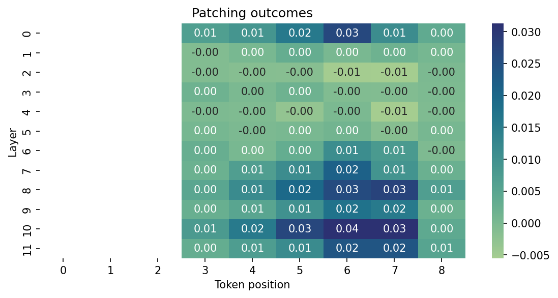
By the looks of this heatmap, activations after attention scoring in the tenth layer of the model seem particularly sensitive to changes between clean and corrupted tokens. Other layers also register this change and could therefore be worth investigating, but the tenth layer scores the highest. Might this be the location where the model has learned something about the difference between “.” and “!”?
9.4.4. Steering the model#
Let’s investigate. Below, we’ll attempt to modify the activations at this layer in hopes that we can alter the model’s behavior. If we can steer the model towards generating text with one token or another, that would be further evidence that we’ve been able to isolate where it has learned a relationship between “.” and “!”.
First, let’s move the model back to a CPU. This isn’t strictly necessary, but
TransformerLens defaults to GPUs when it can find them, and not all of the
following functionality works with that setup.
model.to("cpu")
Moving model to device: cpu
HookedTransformer(
  (embed): Embed()
  (hook_embed): HookPoint()
  (pos_embed): PosEmbed()
  (hook_pos_embed): HookPoint()
  (blocks): ModuleList(
    (0-11): 12 x TransformerBlock(
      (ln1): LayerNormPre(
        (hook_scale): HookPoint()
        (hook_normalized): HookPoint()
      )
      (ln2): LayerNormPre(
        (hook_scale): HookPoint()
        (hook_normalized): HookPoint()
      )
      (attn): Attention(
        (hook_k): HookPoint()
        (hook_q): HookPoint()
        (hook_v): HookPoint()
        (hook_z): HookPoint()
        (hook_attn_scores): HookPoint()
        (hook_pattern): HookPoint()
        (hook_result): HookPoint()
      )
      (mlp): MLP(
        (hook_pre): HookPoint()
        (hook_post): HookPoint()
      )
      (hook_attn_in): HookPoint()
      (hook_q_input): HookPoint()
      (hook_k_input): HookPoint()
      (hook_v_input): HookPoint()
      (hook_mlp_in): HookPoint()
      (hook_attn_out): HookPoint()
      (hook_mlp_out): HookPoint()
      (hook_resid_pre): HookPoint()
      (hook_resid_mid): HookPoint()
      (hook_resid_post): HookPoint()
    )
  )
  (ln_final): LayerNormPre(
    (hook_scale): HookPoint()
    (hook_normalized): HookPoint()
  )
  (unembed): Unembed()
)
With this done, we define a function to produce a steering vector. The idea here is that, at a given point in the network, we access the model’s activations for two tokens. Then, using these activations we make a new vector that represents the tokens’ relationship. That vector is what we’ll send to the model to alter its activations.
You’ll likely recognize the logic here. It’s the first step in the analogy setup we used for static embeddings. Once we get the activations for each token, we simply subtract one from the other to define their relationship.
def make_steering_vector(clean, corrupt, name = None, model = model):
    """Make a steering vector from two tokens.

    Parameters
    ----------
    clean : str
        Clean token
    corrupt : str
        Corrupt token
    name : str
        Name key for the model cache
    model : tl.HookedTransformer
        A hooked model

    Returns
    -------
    steering_vector : torch.Tensor
        A steering vector of size (1, n_dim)
    """
    # Generate vectors for each token
    vectors = []
    for tok in (clean, corrupt):
        _, cache = model.run_with_cache(tok)

        # Extract the activations at a specified layer
        vectors.append(cache[name])

    # Unpack the tokens and subtract the second from the first to define a
    # relationship between the two
    clean, corrupt = vectors
    steering_vector = clean - corrupt

    # Return the results
    return steering_vector[:, 1, :]
With this function defined, we isolate the layer we’re interested in and send our two tokens as arguments.
layer_id = 10
name = tl.utils.get_act_name("attn_out", layer_id)
steering_vector = make_steering_vector(".", "!", name = name)
Finally, we write our own hook. During a forward pass, the model calls this
function when it reaches the component stored at name above. What the
function does is extremely simple: it adds the steering vector to the model
activations. Again, this is just the second step in the analogy setup for
static embeddings.
We also supply an optional coef parameter. As we’ll see below, this helps us
control the effect our steering vector has on the activations.
def steer(activations, hook, steering_vector = None, coef = 1.0):
    """Modify activations with a steering vector.

    Parameters
    ----------
    activations : torch.Tensor
        Model activations
    hook : Any
        Required for compatability with PyTorch but unused
    steering_vector : torch.Tensor
        The steering vector
    coef : float
        A coefficient for scaling the steering vector

    Returns
    -------
    steered : torch.Tensor
        Steered activations
    """
    if steering_vector is None:
        return activations

    return activations + steering_vector * coef
Now, we define a partial function for the hook. All this does is build a new function with some default arguments; the only arguments needed now are ones for activations and the hook, and the model takes care of both of them itself. When we instantiate this partial function, we’ll also modify the coefficient argument. Using a negative coefficient will steer the model towards corrupted output. If we’ve isolated the relationship between “.” and “!” correctly, we’ll see more of the latter tokens.
hook = partial(steer, steering_vector = steering_vector, coef = -3.5)
Time to generate text. Below, we set up a for loop that covers two routines: hooking the model and running it without the hook. That is, we steer it, then we don’t. First, we’ll run this without any sampling.
prompt = "The sky is blue"
for do_hook in (True, False):
    # First, reset all hooks. Then, if we're running with a hook, register it
    model.reset_hooks()
    if do_hook:
        model.add_hook(name = name, hook = hook)

    # Generate text. Note that the hooked model has slightly different
    # parameters for its `.generate()` method
    outputs = model.generate(
        prompt,
        max_new_tokens = 1,
        do_sample = False,
        stop_at_eos = True,
        eos_token_id = model.tokenizer.eos_token_id,
        verbose = False
    )

    # What do we get?
    print(f"Hooked: {do_hook}")
    print(f"Output: {outputs}\n-------")
Hooked: True
Output: The sky is blue!
-------
Hooked: False
Output: The sky is blue,
-------
Promising… But what about with sampling?
model.reset_hooks()
model.add_hook(name = name, hook = hook)

outputs = model.generate(
    prompt,
    max_new_tokens = 50,
    do_sample = True,
    temperature = 0.75,
    top_p = 0.75,
    freq_penalty = 2,
    stop_at_eos = True,
    eos_token_id = model.tokenizer.eos_token_id,
    verbose = False
)
print(outputs)
The sky is blue and the moon is pink! You have arrived at your destination! Now let's get started.

Beware of Star Spangled Bodies!! The way you are greeted by a Star Spangled body will be a delight to behold, and they
Even more promising. Let’s crank the effect of the steering vector way up.
hook = partial(steer, steering_vector = steering_vector, coef = -8.5)
model.reset_hooks()
model.add_hook(name = name, hook = hook)
…and conclude with a final prompt.
prompt = "I had an okay time"
outputs = model.generate(
    prompt,
    max_new_tokens = 50,
    do_sample = True,
    temperature = 0.75,
    top_p = 0.8,
    freq_penalty = 2,
    stop_at_eos = True,
    eos_token_id = model.tokenizer.eos_token_id,
    verbose = False
)
print(outputs)
I had an okay time reading the book! It was awesome! I would recommend this to anyone that loves to read!!!!

One of my favorite books for children and young adults! Amazing story, great art, and very well written!!! Great book!!! The illustrations are